Assessing Studies Based on Multiple Regression
SW Chapter 9
Spring 2026
Learning Objectives
By the end of this chapter, you will be able to:
- Define internal validity and external validity
- Identify five threats to internal validity
- Explain how each threat causes bias or incorrect inference
- Propose solutions to each threat
- Distinguish between causal inference and forecasting objectives
Aside: Linear Probability Models
What if the dependent variable is binary (0/1)?
\[y_i = \beta_0 + \beta_1 x_{1i} + \cdots + \beta_k x_{ki} + u_i\]
If \(y\) only takes values 0 and 1: \(\; E(y|\mathbf{x}) = P(y = 1|\mathbf{x}) = \beta_0 + \beta_1 x_1 + \cdots + \beta_k x_k\)
\(\Rightarrow\) Coefficients measure the change in probability that \(y = 1\) for a one-unit change in \(x_j\)
Limitations: predicted probabilities can fall outside \([0, 1]\); necessarily heteroskedastic (always use robust SEs)
Advantages: easy to estimate and interpret; works naturally with multiple regression tools (controls, IV, fixed effects)
When Is the LPM Appropriate?
The LPM works well when:
- Predicted probabilities are not very high or very low (no strict rule)
- You care about average marginal effects, not predicting exact probabilities
- Your regressors are mostly categorical (dummy variables, interactions)
The LPM is less appropriate when:
- Many predicted probabilities are near 0 or 1 (e.g., rare events)
- You need the predicted probabilities themselves (e.g., for classification or risk scoring)
Bottom line: - For causal inference — which is our focus — the LPM is a perfectly good tool. - Angrist & Pischke (Mostly Harmless Econometrics) argue it gives you the right average effects without the complexity of nonlinear models. - More formal alternatives (probit, logit) exist but are beyond ECON3500. - You will use the LPM in Lab 6!
Internal and External Validity
What Is Validity?
Validity = Do we believe the results of our estimation?
Did we learn what we set out to learn?
- Did we estimate the causal impact of class size on test scores?
- Did we correctly measure the association between marital status and wages?
We need a framework for evaluating whether a study is useful for answering a particular question.
What are the threats to validity?
Two Dimensions of Validity
Internal Validity
The statistical inferences about causal effects are valid for the population being studied.
External Validity
The statistical inferences can be generalized from the population and setting studied to other populations and settings.
“Setting” = the legal, policy, and physical environment and related salient features.
External Validity Example: Seattle Minimum Wage
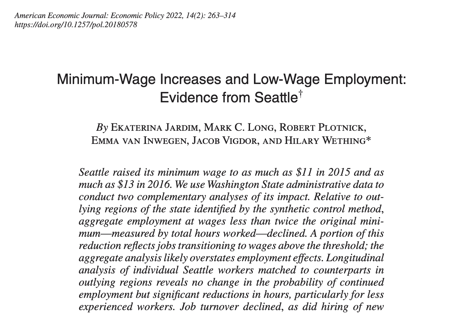
Question: A study finds Seattle’s $15 minimum wage reduced hours for low-wage workers (Jardim et al. 2022, AEJ: Economic Policy). Would we expect the same result elsewhere?
Jardim et al. (2022), AEJ: Economic Policy
Threats to External Validity
Assessing external validity requires detailed substantive knowledge and judgment on a case-by-case basis.
Same example: Seattle’s $15 minimum wage and hours worked. What should we ask before generalizing?
- Differences in populations
- Seattle’s low-wage workforce: tech-adjacent, high cost of living
- Rural Vermont? Mississippi? Workers face very different outside options
- Differences in settings
- Seattle’s booming economy may have cushioned the shock
- Different state labor laws, tipped wage rules, enforcement
- Differences in labor markets
- Urban labor markets are less concentrated — more employers competing for workers
- Research shows more concentrated (rural) labor markets may respond differently to minimum wage increases (Azar et al. 2023)
There is no mechanical test for external validity — it requires judgment.
Internal Validity: Two Requirements
Estimates are internally valid if:
- The estimator is consistent (or unbiased)
- Confidence intervals have correct coverage — in at least 95% of samples, the 95% CI contains the true parameter
The Rest of This Chapter
We focus on threats to internal validity: things that can make our regression estimates misleading for the population we’re studying.
Five Threats to Internal Validity
Overview
Five threats to the internal validity of regression studies:
- Omitted variable bias
- Wrong functional form
- Errors-in-variables bias (measurement error)
- Sample selection bias
- Simultaneous causality bias
All five imply that \(E(u_i | X_{1i}, \ldots, X_{ki}) \neq 0\)
\(\Rightarrow\) Conditional mean independence fails
\(\Rightarrow\) OLS is biased and inconsistent
Quick Review
- Biased: \(E[\hat{\beta}] \neq \beta\) — on average across samples, our estimator gets the wrong answer
- Consistent: as \(n \rightarrow \infty\), \(\hat{\beta}\) converges in probability to \(\beta\) — more data gets you closer to the truth. When an estimator is inconsistent, more data doesn’t fix the problem.
Three Categories of Threats
When you encounter a potential threat, classify it:
| Category | What goes wrong | Severity |
|---|---|---|
| 1. Affects consistency of \(\hat{\beta}\) | Estimator converges to wrong value | Most serious |
| 2. Affects inference but not consistency | CIs have wrong coverage; \(\hat{\beta}\) is still consistent | Serious |
| 3. Increases imprecision only | Larger SEs, but \(\hat{\beta}\) unbiased and CIs correct | Least serious |
- Categories 1 and 2 are actual threats to validity
- Category 3 makes estimates imprecise but standard errors properly reflect that imprecision
1. Omitted Variable Bias
We know this one! OVB arises if an omitted variable is both (1) a determinant of \(Y\), and (2) correlated with at least one included regressor.
With control variables included, are there still omitted factors that are not adequately controlled for? Is the error term correlated with the variable of interest even after we have included the control variables?
Solutions:
- If the omitted variable can be measured: include it as an additional regressor
- If you have adequate controls (conditional mean independence plausibly holds): include them
- Run a randomized controlled experiment — if \(X\) is randomly assigned, \(E(u|X) = 0\)
- Use panel data (Ch10) or instrumental variables (Ch12) — coming soon!
2. Wrong Functional Form
Arises if the functional form is incorrect — for example, an interaction term is incorrectly omitted; then inference on causal effects will be biased.
Solutions to functional form misspecification:
- Continuous \(Y\): use the appropriate nonlinear specifications in \(X\) (logarithms, interactions, etc. — Ch8)
- Discrete \(Y\) (e.g., binary): use a linear probability model (as in Lab 6), or more formally, probit or logit (beyond ECON3500)
Note: This issue is rarely our biggest problem in regression analysis.
3. Errors-in-Variables Bias
So far we’ve assumed \(X\) is measured without error. In reality, economic data often have measurement error:
- Data entry errors in administrative data
- Recollection errors in surveys (“When did you start your current job?”)
- Ambiguous questions (“What was your income last year?” — before or after tax?)
- Intentionally false responses (“What is the current value of your financial assets?” “How often do you drink and drive?”)
Example
What sort of problem does this create?
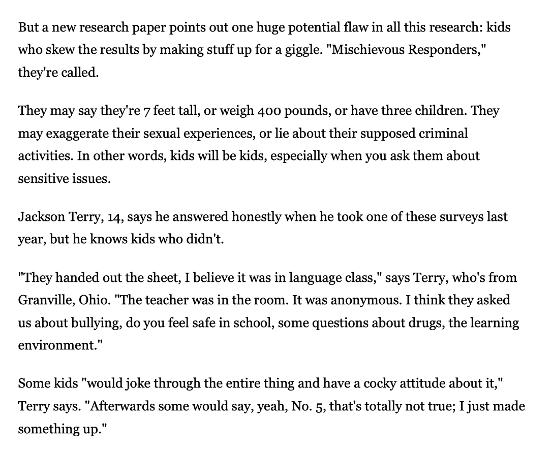
Example of potentially inaccurate self-reported survey responses
- Self-reported survey data can be wrong because respondents misremember, misunderstand, or make things up
- For sensitive questions, the error may be systematic, not purely random
- That means measurement error in survey data is often not classical
Source: Anya Kamenetz, “Mischievous Responders’ Confound Research On Teens,” NPR, May 22, 2014.
Where and What Kind?
Measurement error can occur in the dependent variable or independent variables.
And it can be classical (random) or non-classical (systematic).
| Classical (random) | Non-classical (systematic) | |
|---|---|---|
| Dependent variable | Minor problem — larger variance | Serious problem — bias |
| Independent variable | Attenuation bias | Serious problem — bias |
Classical Errors-in-Variables (CEV) Assumption
The measurement error is uncorrelated with the true value: \(\text{Cov}(w_i, X^*_i) = 0\)
Measurement Error in \(Y\)
Suppose we observe \(y_i\) but the true value is \(y^*_i\):
\[y_i = y^*_i + e_i\]
The population regression is:
\[y^*_i = \beta_0 + \beta_1 x_1 + \cdots + \beta_k x_k + u_i\]
What we actually estimate:
\[y_i = \beta_0 + \beta_1 x_1 + \cdots + \beta_k x_k + \underbrace{(u_i + e_i)}_{\text{new error term}}\]
If \(e_i\) is uncorrelated with the \(X\)’s, the coefficients are still unbiased — the error term just has more variance, so standard errors are larger.
Measurement error in \(Y\) under CEV: not a big deal.
Measurement Error in \(X\): Setup
The true model is:
\[Y_i = \beta_0 + \beta_1 X^*_i + u_i\]
We observe \(X_i = X^*_i + w_i\) instead of \(X^*_i\), where \(E[w_i] = 0\).
Assumptions (classical errors-in-variables):
- \(\text{Cov}(w_i, u_i) = 0\) — measurement error uncorrelated with other omitted factors
- \(\text{Cov}(w_i, X^*_i) = 0\) — measurement error uncorrelated with the true value ← the CEV assumption
- \(\text{Cov}(X^*_i, u_i) = 0\) — no traditional OVB
Why Is This a Problem?
The key insight: even though \(\text{Cov}(w_i, X^*_i) = 0\), the measurement error \(w_i\) is correlated with the observed \(X_i\).
\[\text{Cov}(X_i, w_i) = \text{Cov}(X^*_i + w_i, \; w_i)\]
\[= \underbrace{\text{Cov}(X^*_i, w_i)}_{= \; 0 \text{ by CEV}} + \text{Cov}(w_i, w_i)\]
\[= \text{Var}(w_i) = \sigma^2_w\]
The observed regressor \(X_i\) is correlated with the measurement error, which is part of the composite error term. This violates conditional mean independence.
Formal Derivation of Measurement Error (1/2)
\[\hat{\beta}_1 = \frac{\text{Cov}(X_i, Y_i)}{\text{Var}(X_i)}\]
\[= \frac{\text{Cov}(X^*_i + w_i, \; \beta_0 + \beta_1 X^* + u_i)}{\text{Var}(X^*_i + w_i)}\]
Expanding the numerator:
\[= \frac{\text{Cov}(X^*_i, \beta_0) + \text{Cov}(X^*_i, \beta_1 X^*_i) + \text{Cov}(w_i, \beta_0) + \text{Cov}(w_i, \beta_1 X^*) + \text{Cov}(w_i, u_i)}{\text{Var}(X^*_i) + \text{Var}(w_i) + 2\text{Cov}(X^*_i, w_i)}\]
Formal Derivation of Measurement Error (2/2)
Applying our assumptions (\(\text{Cov}(w, X^*) = 0\), \(\text{Cov}(w, u) = 0\)):
\[= \frac{0 + \beta_1 \text{Var}(X^*_i) + 0 + 0 + 0}{\text{Var}(X^*_i) + \text{Var}(w_i) + 0}\]
\[= \beta_1 \cdot \frac{\text{Var}(X^*_i)}{\text{Var}(X^*_i) + \text{Var}(w_i)}\]
Attenuation Bias: The Result
\[\hat{\beta}_1 = \beta_1 \cdot \frac{\text{Var}(X^*_i)}{\text{Var}(X^*_i) + \text{Var}(w_i)}\]
The fraction on the right is between 0 and 1. So:
- If \(\beta_1 > 0\): estimate is biased toward zero (too small)
- If \(\beta_1 < 0\): estimate is biased toward zero (too close to zero)
Attenuation Bias
Classical measurement error in a regressor always biases the coefficient toward zero — making the estimated effect look smaller than it truly is.
Attenuation Bias: Intuition
Why does this happen?
- \(X_i\) has a higher variance than the true \(X^*_i\) (the noise adds spread)
- When \(X_i\) moves, \(Y\) doesn’t always respond — because \(Y\) only responds to movements in \(X^*\)
- The regression sees changes in \(X\) that are not related to \(Y\)
- It concludes: “the effect of \(X\) on \(Y\) must be small”
Practical implication: If we think there’s measurement error in \(X\), our estimate is a lower bound on the true magnitude.
What If CEV Doesn’t Hold?
Sometimes the classical assumption is unlikely:
- People with high incomes under-report and people with low incomes over-report
- \(\Rightarrow \text{Cov}(\text{income}, \text{error}) \neq 0\)
- People are less accurate about their age as they get older
- \(\Rightarrow \text{Cov}(\text{age}, \text{error}) \neq 0\)
When CEV fails:
- The direction of bias is ambiguous — no longer necessarily toward zero
- Interpreting the impact is more complicated (beyond ECON3500)
Summary of Measurement Error
- Dependent variable (classical): Don’t worry too much — OLS still BLUE, just larger variance
- Independent variable (classical): OLS no longer BLUE — attenuation bias
- We can still sign our magnitudes (e.g., “Returns to education are at least 10%”)
- Independent variable (non-classical): OLS no longer BLUE — bias in ambiguous direction
- Better data always helps! Use administrative records instead of survey self-reports when possible.
- Use instrumental variables (later)
4. Missing Data and Sample Selection Bias
Data are often missing. Whether this introduces bias depends on why the data are missing:
| Case | Data missing because of… | Bias? |
|---|---|---|
| 1 | Random chance | No |
| 2 | Values of \(X\) | No |
| 3 | Values of \(Y\) or \(u\) | Yes |
- Cases 1 and 2: standard errors are larger, but \(\hat{\beta}\) is unbiased
- Case 3: introduces sample selection bias
Case 1: Missing at Random
Suppose you survey 100 workers and record answers on paper — but your dog eats 20 response sheets (selected at random) before you enter them.
This is equivalent to having a random sample of 80 workers.
Your dog didn’t introduce any bias!
Knowledge Check
A server crash deletes 30% of your dataset at random. Should you worry about bias?
No — this is Case 1. You lose precision (larger SEs) but no bias.
Case 2: Missing Based on \(X\)
Suppose you’re studying the effect of education on wages, but you restrict your sample to workers under age 30.
- You can’t say anything about older workers
- But restricting to younger workers doesn’t introduce bias for the under-30 population
- This is equivalent to having missing data where data are missing based on \(X\) (age)
More generally: if data are missing based only on values of \(X\), the missing data don’t bias OLS. (It does limit external validity — you can’t generalize beyond that subgroup.)
Case 3: Missing Based on \(Y\) or \(u\)
This does introduce bias. This is sample selection bias.
Sample selection bias arises when a selection process:
- Influences the availability of data, and
- Is related to the dependent variable
In DAG terms: this is collider bias — conditioning on a variable that is caused by both \(X\) and \(Y\) (recall Ch 8b slides).
The Key Question
Ask yourself: “Would the reason someone is missing from my data be correlated with the outcome I’m trying to measure?” If yes \(\rightarrow\) sample selection bias.
Example: Height of Undergraduates
You want to estimate the mean height of undergraduates.
You collect data by standing outside the basketball team’s locker room and recording the height of undergraduates who enter.
Is this a good design?
- No
- You’ve sampled individuals in a way that is related to the outcome \(Y\) (height)
- This results in bias — your estimate will be too high
Example: Mutual Fund Performance
Question: Do actively managed mutual funds outperform “hold-the-market” index funds?
Design:
- Sample: mutual funds available to the public today
- Data: returns for the preceding 10 years
- Compare: average 10-year return vs. S&P 500
Is there sample selection bias?
Yes — funds that performed poorly went out of business and are not in today’s sample.
The surviving funds are the “basketball players” of mutual funds.
This is called survivorship bias — the surviving funds are the “basketball players” of mutual funds.
Being managed and in our sample means the fund outperformed failed managed funds \(\Rightarrow \text{Cov}(\text{managedfund}_i, \; u_i) \neq 0\) \(\Rightarrow\) OLS is biased
Example: Returns to Education
Question: What is the return to an additional year of education among college graduates?
Design:
- Sample: employed college graduates (so we have wage data)
- Regress: \(\ln(\text{earnings})\) on years of education
Is there sample selection bias?
Yes — we only observe wages for people who are employed. Employment is related to the outcome (wages/earnings potential), so the sample is not representative.
Solutions to Sample Selection Bias
Collect data properly — design sampling to avoid selection
- Basketball: true random sample from enrollment records
- Mutual funds: sample funds available at the beginning of the period (include failed funds)
- Returns to education: sample college graduates, not just employed workers
Randomized controlled experiment
Model the selection process and estimate it (advanced — not in ECON3500)
5. Simultaneous Causality Bias
So far we’ve assumed \(X\) causes \(Y\). But what if \(Y\) also causes \(X\)?
This is simultaneous causality (or “reverse causality”). Remember: the “A” in DAG stands for acyclic — DAGs cannot represent simultaneity (Ch 8b slides).
Example: Class size effect
- Low STR \(\rightarrow\) better test scores (the effect we want)
- But: districts with low test scores may receive extra resources \(\rightarrow\) also get low STR (political process)
What does this mean for a regression of TestScore on STR?
The coefficient on STR reflects both directions of causality — it’s biased.
Solutions to Simultaneous Causality Bias
Randomized controlled experiment — because \(X_i\) is chosen at random, there is no feedback from \(Y\) to \(X\) (assuming perfect compliance)
Develop a complete model of both directions of causality — this is the approach behind large macroeconomic models (e.g., Federal Reserve). Extremely difficult in practice.
Instrumental variables regression — estimate the causal effect of \(X\) on \(Y\) while ignoring the feedback from \(Y\) to \(X\) (coming later!)
Summary: Five Threats to Internal Validity
| Threat | What Happens | Consequence | Solutions |
|---|---|---|---|
| 1. OVB | Omitted variable correlated with \(X\) and determines \(Y\) | Biased, inconsistent | Add controls, RCT, IV, panel data |
| 2. Wrong functional form | Incorrect specification (missing interactions, nonlinearities) | Biased | Logs, quadratics, interactions (Ch8) |
| 3. Measurement error | \(X\) or \(Y\) measured with error | Attenuation bias (classical); ambiguous bias (non-classical) | Better data, IV |
| 4. Sample selection | Data missing based on \(Y\) or \(u\) | Biased, inconsistent | Better sampling design, RCT |
| 5. Simultaneous causality | \(Y\) causes \(X\) and \(X\) causes \(Y\) | Biased, inconsistent | RCT, IV |
Forecasting vs. Causal Inference
Forecasting vs. Causal Inference
| Causal Inference | Forecasting | |
|---|---|---|
| Goal | Estimate effect of changing \(X\) on \(Y\) | Predict \(Y\) given observed \(X\)’s |
| What matters most | Unbiased \(\hat{\beta}\) | Good fit (\(\bar{R}^2\)) |
| OVB | Critical problem | Not a problem! |
| Coefficient interpretation | Very important | Not important |
| External validity | Important for generalization | Paramount — model must hold in new data |
Don’t Confuse the Two
A model with high \(R^2\) and biased coefficients might be great for forecasting but useless for policy. A model with unbiased coefficients and low \(R^2\) might be ideal for causal inference but poor for prediction.
Knowledge Check: Identify the Threat
For each scenario, identify the primary threat to internal validity:
1. A study of returns to education uses IQ as a proxy for ability, but IQ tests are noisy measures of true ability.
\(\rightarrow\) Errors-in-variables bias (measurement error in \(X\)) — attenuation bias on the IQ coefficient
2. A study of the effect of police on crime finds that cities with more police have more crime.
\(\rightarrow\) Simultaneous causality — high-crime cities hire more police
3. A study of job training effects on wages only observes wages for people who are employed after training.
\(\rightarrow\) Sample selection bias — employment status is related to the outcome (wages)
Key Takeaways
Measurement error in \(X\) (classical) causes attenuation bias — estimates are too small in magnitude
Sample selection bias arises when data are missing because of \(Y\), not because of \(X\) or random chance
Simultaneous causality is hard to solve without experiments or instrumental variables
Looking Ahead
Panel data (Ch10) and instrumental variables (Ch12) are direct responses to OVB and simultaneous causality.
ECON3500 | Chapter 9