Causal Diagrams and Identifying Causal Effects

Directed Acyclic Graphs (DAGs)

ECON3500: Econometrics and Applications

Spring 2026

Learning Objectives

By the end of this lecture, you will be able to:

Draw and interpret directed acyclic graphs (DAGs)
Identify causal paths, backdoor paths, and colliders
Determine which variables to control for to identify a causal effect
Explain why controlling for the wrong variables can bias your estimates
Apply DAG logic to real research questions

Reading

Huntington-Klein, The Effect: Chapters 6, 7, and 8 (available free at theeffectbook.net)

What Is Causality?

The Data Generating Process

Every dataset we observe is produced by a data generating process (DGP) — the real-world laws, behaviors, and institutions that determine the values we see.

Our challenge as econometricians:

We observe the data, not the DGP
Multiple DGPs could produce the same data patterns
We need a framework for reasoning about which variation in our data answers our research question

Identification

Identification is the process of figuring out what part of the variation in your data answers your research question.

Association vs. Causation

Association

Two variables move together (correlation). \(X\) and \(Y\) are related statistically.

Causation

Changing \(X\) causes \(Y\) to change. Formally: if we could intervene to change \(X\), the distribution of \(Y\) would change as a result.

Association: Useful for prediction, not necessarily for policy
Causation: Required for policy impact, program evaluation, treatment effects

The Framework: Causal Diagrams (DAGs)

A directed acyclic graph (DAG) is a visual representation of a data generating process. Every word in the name matters:

Directed: Arrows point in one direction — from cause to effect
Acyclic: No cycles — you can never follow arrows and end up back where you started
Graph: A diagram with nodes (variables) and edges (arrows)

The acyclic part is a real constraint: DAGs assume causality flows forward. If \(X\) causes \(Y\) and \(Y\) simultaneously causes \(X\), a DAG can’t represent that. (We’ll return to this when we discuss simultaneity.)

Key insight: Once we draw the DAG, we can mechanically determine which variables to control for to identify a causal effect.

Important assumption

Every variable and arrow that is not on the diagram is an assumption we’re making. Drawing a DAG forces you to be explicit about your identifying assumptions.

Drawing and Reading DAGs

DAG Basics: Nodes and Arrows

Node: A variable in the system.

Each circle represents a variable — either observed or unobserved.

Arrow: \(X \rightarrow Y\) means “\(X\) causes \(Y\).”

Direction matters (from cause to effect)
\(X\) is a parent (ancestor) of \(Y\)
\(Y\) is a child (descendant) of \(X\)

Example: Class Size and Student Achievement

Variables:

\(X\) = Class Size, \(Y\) = Test Scores, \(Z\) = Wealth

Causal arrows:

Wealth → Class Size (wealthy areas have smaller classes)
Wealth → Test Scores (wealthier students score higher)
Class Size → Test Scores (smaller classes improve learning)

How to Build a DAG

Step-by-Step DAG Construction

Building a DAG is a structured process (HK, The Effect, Ch. 6):

Step 1: List all relevant variables. What might cause your treatment? What might cause your outcome? What affects both? Cast a wide net.

Step 2: For each pair of variables, ask “does one cause the other?” If yes, draw an arrow from cause to effect. If you draw no arrow, you’re assuming no direct causal link between those variables.

Step 3: Simplify. Remove any variable that is not on any path between your treatment and outcome. If it doesn’t connect \(X\) and \(Y\) (directly or indirectly), it doesn’t affect your identification — so it can be dropped.

Step 4: Determine what to control for. Apply the backdoor criterion to find the minimal set of controls that closes all backdoor paths. (We’ll get to this soon!)

Building DAGs: Handling Correlated Variables

What if two variables are correlated but neither causes the other?

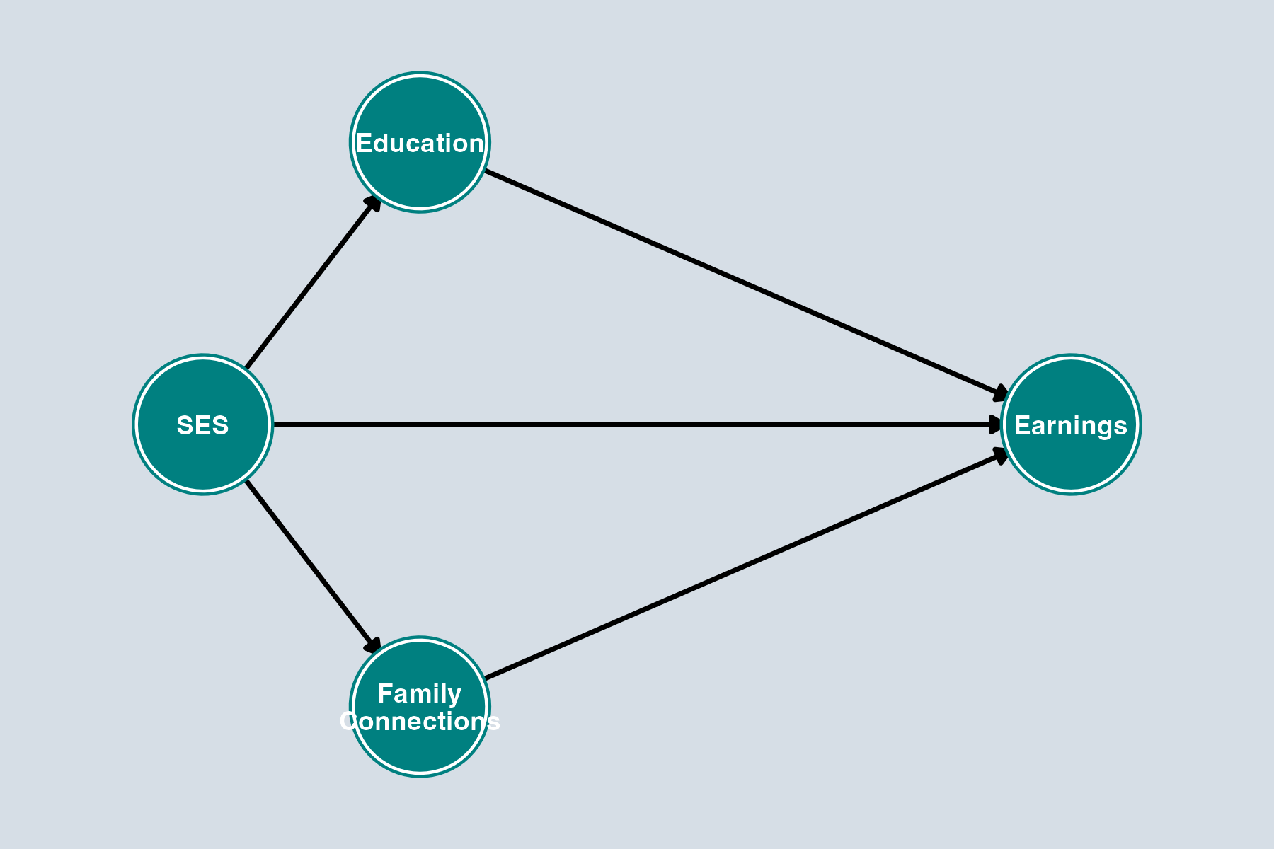
Sometimes you have two variables — say, Income and SES — that are clearly correlated, but you don’t think one directly causes the other.

Solution: Introduce a shared unobserved cause \(U\) that drives both.

\[U \rightarrow \text{Income} \quad \text{and} \quad U \rightarrow \text{SES}\]

This is more honest than arbitrarily picking a direction for the arrow. You’re saying: “something generates both of these, but I don’t need to name it.” In a DAG, draw \(U\) as a gray (unobserved) node with arrows pointing to both variables.

Causal (Front Door) Paths

\(X \rightarrow Y\) (or \(X \rightarrow M \rightarrow Y\))

Direct or indirect effect of \(X\) on \(Y\), with all arrows pointing away from \(X\).

These are good paths — they represent what we want to estimate.

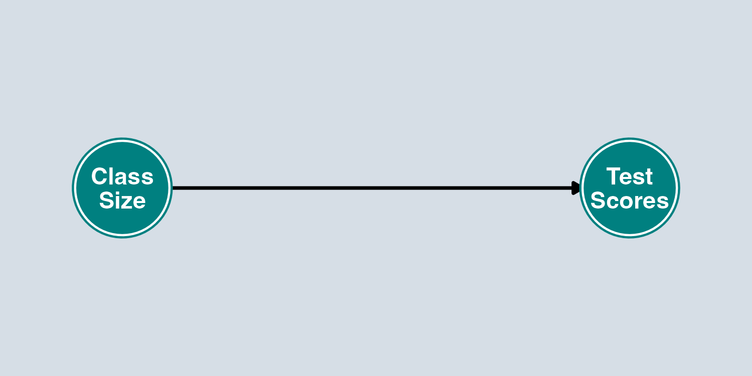
Example: Class Size → Test Scores

Backdoor Paths

\(X \leftarrow Z \rightarrow Y\)

\(X\) and \(Y\) are connected through a common cause \(Z\). These are bad paths — they create confounding.

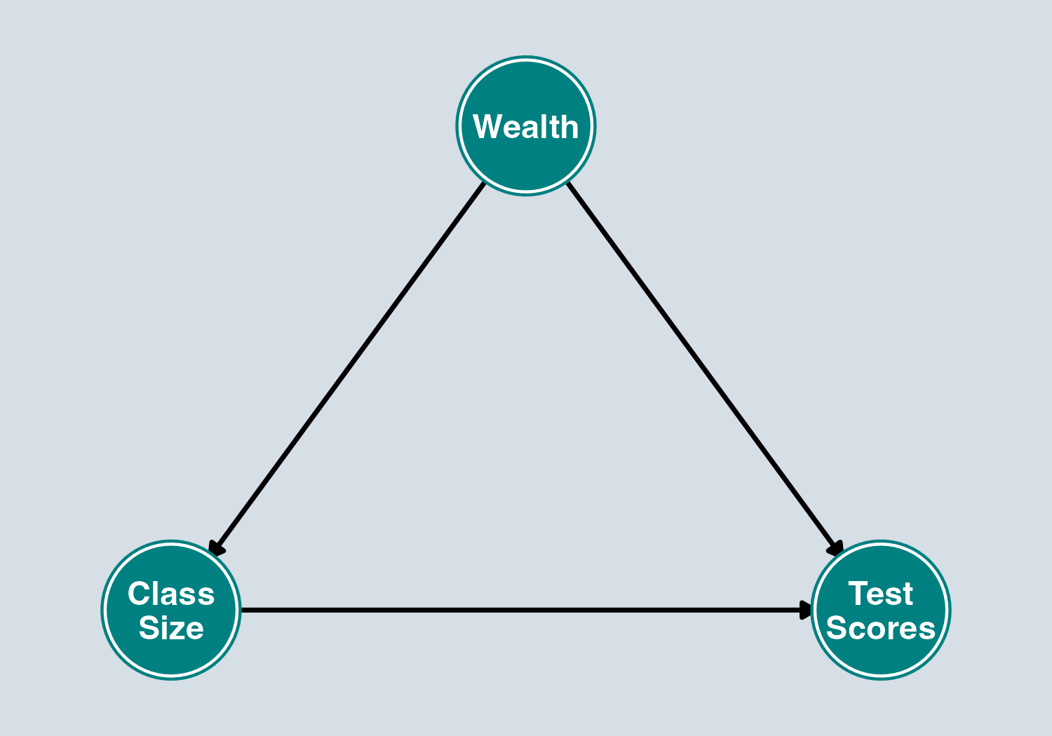
Example: Class Size ← Wealth → Test Scores

Collider Paths

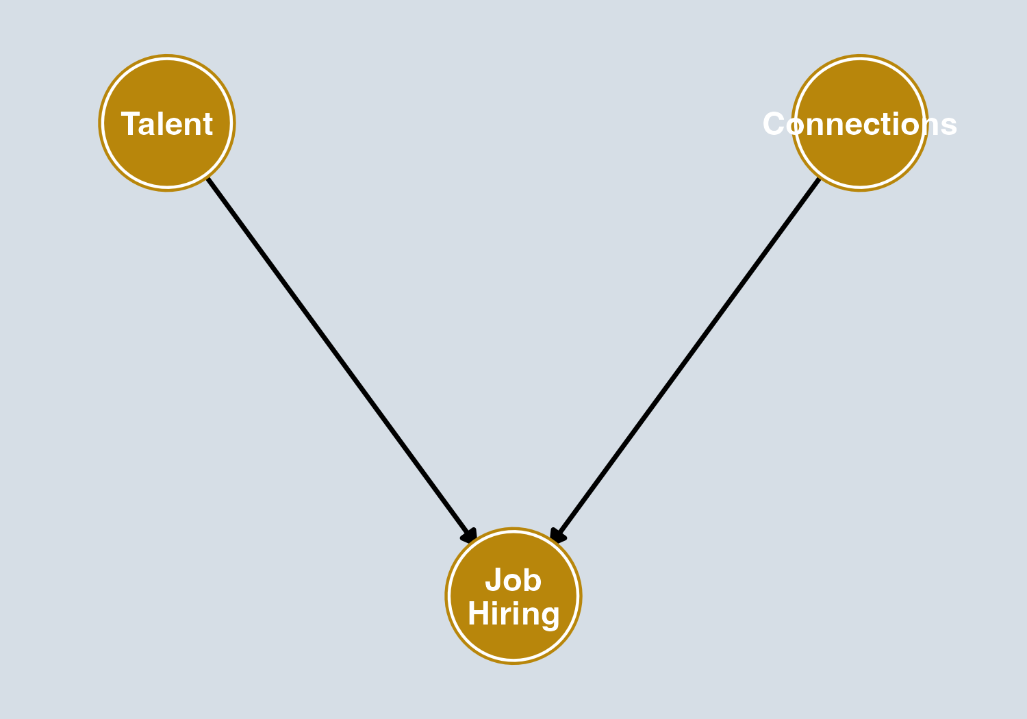
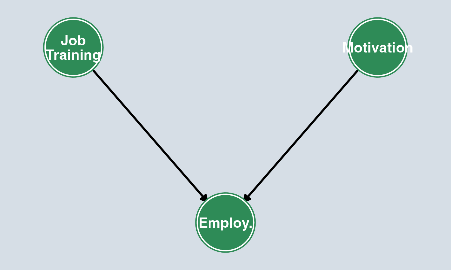
\(X \rightarrow Z \leftarrow Y\)

\(X\) and \(Y\) both cause \(Z\). These paths are closed by default — no confounding flows through them unless we control for \(Z\).

Talent and Connections both cause Job Hiring
The path Talent → Job Hiring ← Connections is closed by default
If we condition on who was hired (control for the collider), the path opens
Among the hired: low Talent becomes correlated with high Connections

What Does “Controlling” Mean?

When we say “control for \(Z\)” in a regression, we are comparing units that have the same value of \(Z\). This removes the variation in \(X\) and \(Y\) that is driven by \(Z\).

In DAG terms: Controlling for a variable blocks all paths that pass through it. This can be good or bad:

Path Type	Default Status	What controlling does
Backdoor (\(X \leftarrow Z \rightarrow Y\))	Open	Closes it → removes bias
Collider (\(X \rightarrow Z \leftarrow Y\))	Closed	Opens it → creates bias
Mediator (\(X \rightarrow Z \rightarrow Y\))	Open	Closes it → blocks the causal effect

Our goal: Close all bad (backdoor) paths while keeping good (causal) paths open — and not accidentally opening closed ones.

Confounding, OVB, and the Backdoor Criterion

Confounding = OVB = Open Backdoor Path

Confounding

When \(X\) and \(Y\) share a common cause \(Z\), they are confounded. A regression of \(Y\) on \(X\) will pick up both the causal effect AND the confounding association.

\[\text{Association} = \underbrace{\text{Causal Effect}}_{\text{Class Size} \rightarrow \text{Scores}} + \underbrace{\text{Confounding Bias}}_{\text{via Wealth}}\]

Remember omitted variable bias from Chapter 6? Every case of OVB is an open backdoor path. The omitted variable creates a backdoor path that stays open, and the bias flows through it into \(\hat{\beta}_1\).

Knowledge Check: Direction of Bias

Think About It

If we regress Test Scores on Class Size without controlling for Wealth, will the class size coefficient be biased up or down?

Answer: The coefficient on class size is biased away from zero (overstates the negative effect).

Wealthy areas → smaller classes AND higher scores
This creates a negative confounding association between class size and scores
The negative confounding reinforces the true negative causal effect, making OLS more negative than the true \(\beta_1\)

The Backdoor Criterion

To identify the causal effect of \(X\) on \(Y\):

Backdoor Criterion

Control for a set of variables \(\mathbf{Z}\) such that:

No variable in \(\mathbf{Z}\) is a descendant of \(X\)
Controlling for \(\mathbf{Z}\) closes all backdoor paths from \(X\) to \(Y\)

In plain language:

Do control for common causes (confounders) — they create open backdoor paths
Don’t control for variables that \(X\) affects — that would block part of the causal effect
Don’t control for colliders — that would open a path that was safely closed

Applying the Criterion: List All Paths

A systematic approach to finding your controls:

List every path connecting \(X\) and \(Y\) (follow arrows in any direction)
Classify each path: Is it a causal (front-door) path or a backdoor path?
Check each path’s status: Is it currently open or closed?
Choose controls to close all open backdoor paths — without opening any closed paths

Example: Class Size and Test Scores

Path	Type	Default	Action
Class Size → Test Scores	Causal	Open	Leave open
Class Size ← Wealth → Test Scores	Backdoor	Open	Control for Wealth

After controlling for Wealth: the only remaining open path is causal. The effect is identified.

What NOT to Control For: Mediators

Bad Control: Mediator

If \(X \rightarrow M \rightarrow Y\), then \(M\) is a mediator. Controlling for \(M\) blocks part of the causal effect of \(X\) on \(Y\).

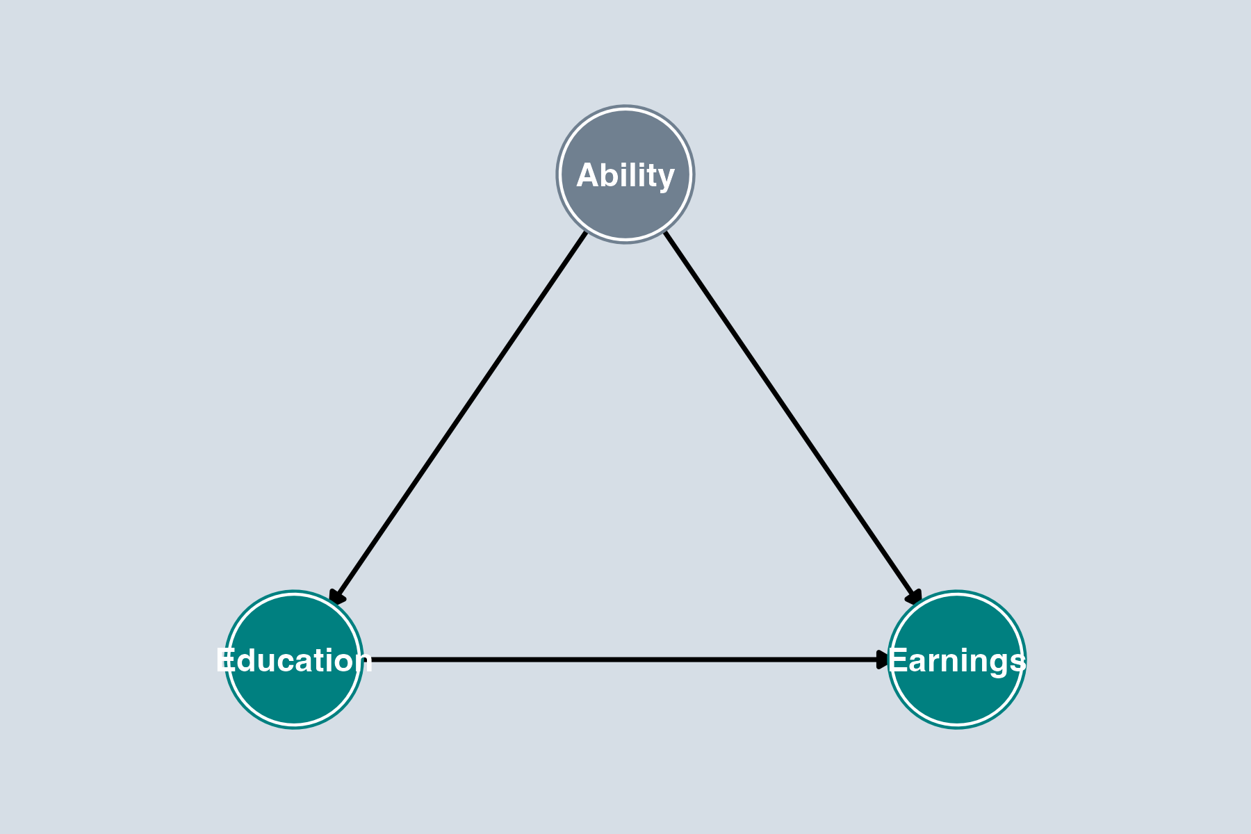
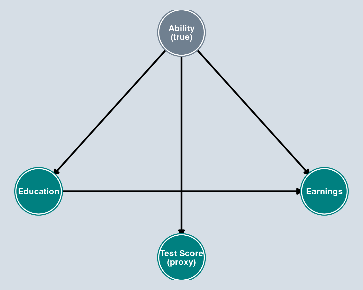
Example: Does education affect earnings?

Education → Job Type → Earnings
If we control for Job Type, we block the indirect effect of education that works through job placement
We’d only estimate the effect of education holding job type fixed — not the total causal effect

Applications: Identifying Causal Effects

Does Education Cause Earnings?

Gray node = unobserved variable

Causal path? Yes: Education → Earnings
Backdoor paths? Yes: Education ← Ability → Earnings
What to control for? Ability

Does Education Cause Earnings? (cont.)

Challenge: Ability is unobserved! We can’t directly control for it.

This is why economists turn to identification strategies — instruments, experiments, panel data — to close backdoor paths when confounders are unobservable.

Does Job Training Improve Employment?

The problem without randomization:

Motivated workers are more likely to sign up for training
Motivated workers are also more likely to find jobs
Backdoor path: Training ← Motivation → Employment

. . .

With an RCT:

Randomly assign workers to training
Now Motivation does not cause Training — that arrow is severed
All backdoor paths are closed by design

Important

This is why randomized controlled trials (RCTs) are the gold standard for causal inference — they eliminate confounding mechanically.

Reverse Causation

Reverse Causation

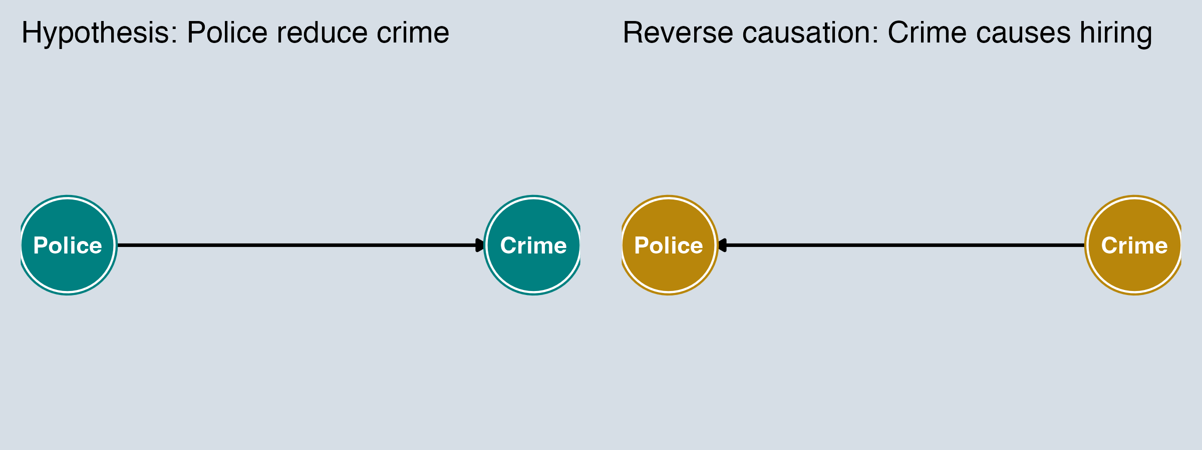
Sometimes the arrow between \(X\) and \(Y\) runs in the opposite direction from what we assume.

We observe a positive correlation between police and crime
Our hypothesis: More police → less crime
The problem: Cities with more crime hire more police

In DAG terms: we’ve drawn the wrong DAG. The true DGP has the arrow reversed — or both arrows exist.

DAGs and Simultaneity

Remember: the “A” in DAG stands for acyclic. DAGs cannot represent simultaneity — when \(X\) causes \(Y\) and \(Y\) simultaneously causes \(X\).

Two approaches when you suspect reverse causation or simultaneity:

Approach 1: Use time subscripts

Separate variables by time period: \(X_t \rightarrow Y_{t+1}\) and \(Y_t \rightarrow X_{t+1}\). This converts a cycle into an acyclic graph — causality flows forward through time. Works well when the feedback loop operates with a lag (e.g., crime this year → police budget next year).

Approach 2: Use instrumental variables

When the relationship is truly simultaneous (e.g., price and quantity in a market), the DAG framework alone can’t solve it. This is where instrumental variables and 2SLS become the right tools — you need an external source of variation that shifts one variable without directly affecting the other. We’ll cover this in detail later in the course.

Measurement Error

Gray = unobserved

Measurement Error

When we can’t perfectly measure a variable in our DAG, we introduce measurement error.

We want to control for Ability to close a backdoor path
We can’t measure Ability directly, so we use a proxy (Test Score)
But Test Score ≠ Ability (noisy measurement)
Controlling for the proxy only partially closes the backdoor path
Result: our estimate is still biased — attenuation bias

Knowledge Checks and Practice

Knowledge Check 1: Health Insurance

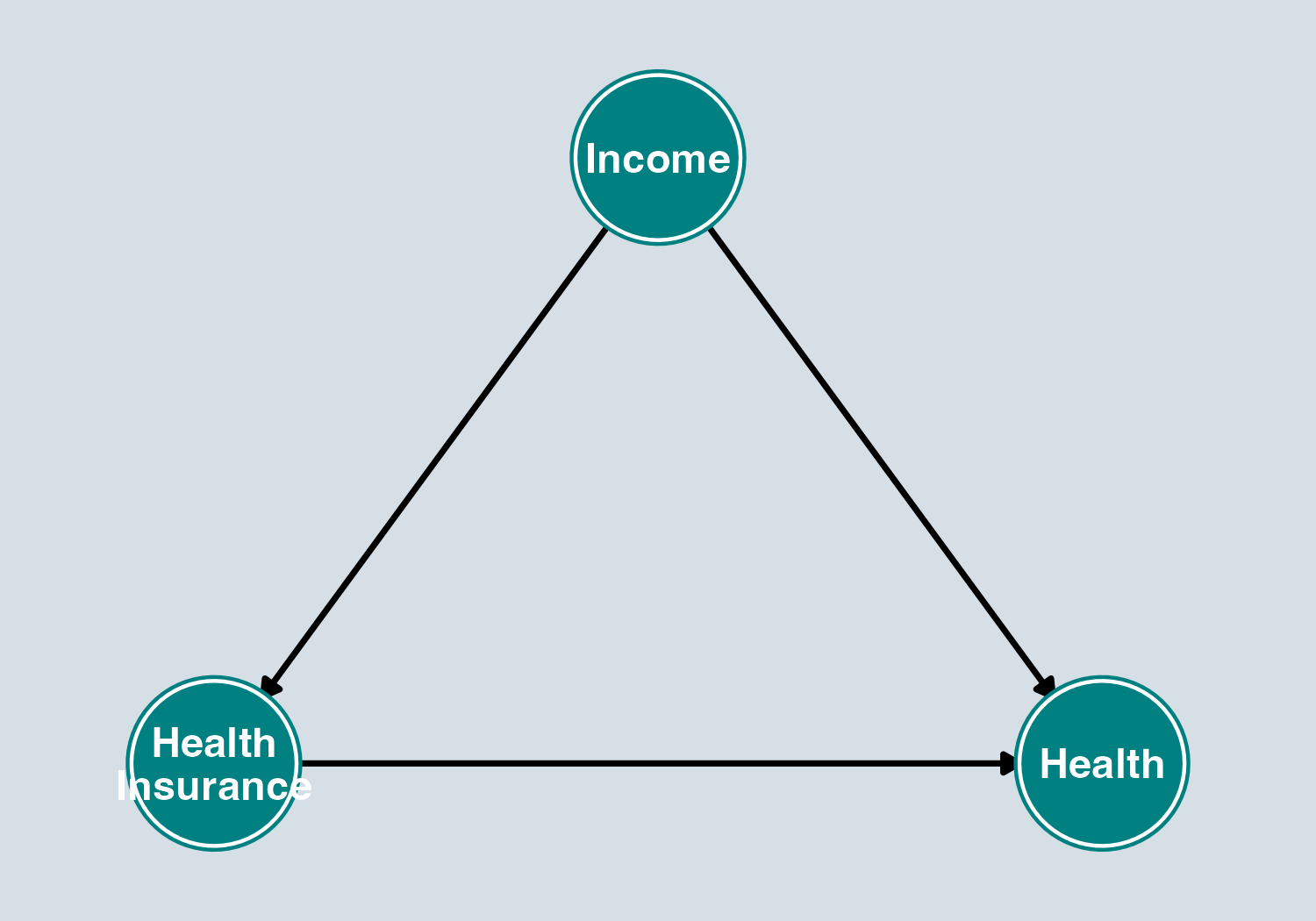
Does Income confound the effect of Health Insurance on Health?

To estimate the effect of Health Insurance on Health, should we control for Income?

Knowledge Check 1: Answer

Answer

There is a backdoor path: Health Insurance ← Income → Health
Income is a common cause of both Health Insurance and Health
So yes, we should control for Income — it’s a confounder

Knowledge Check 2: SES and Earnings

Questions:

What are the backdoor paths from SES to Earnings?
What minimal set of variables should we control for?

Knowledge Check 2: Answer

Answer

Backdoor path: SES ← (shared causes) → Earnings via Family Connections
Controls: Family Connections (to close the backdoor)
- Do NOT control for Education — it is a descendant of SES (mediator)

Case Study: Does Wine Improve Heart Health?

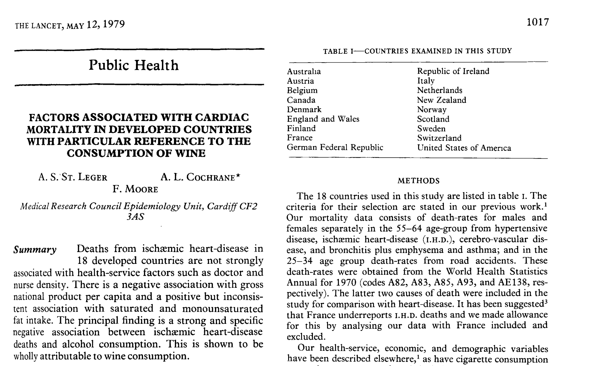
St Leger, Cochrane, & Moore (1979). The Lancet.

In 1979, researchers found a strong negative association between wine consumption and heart disease across 18 developed countries.

The French Paradox Goes Mainstream

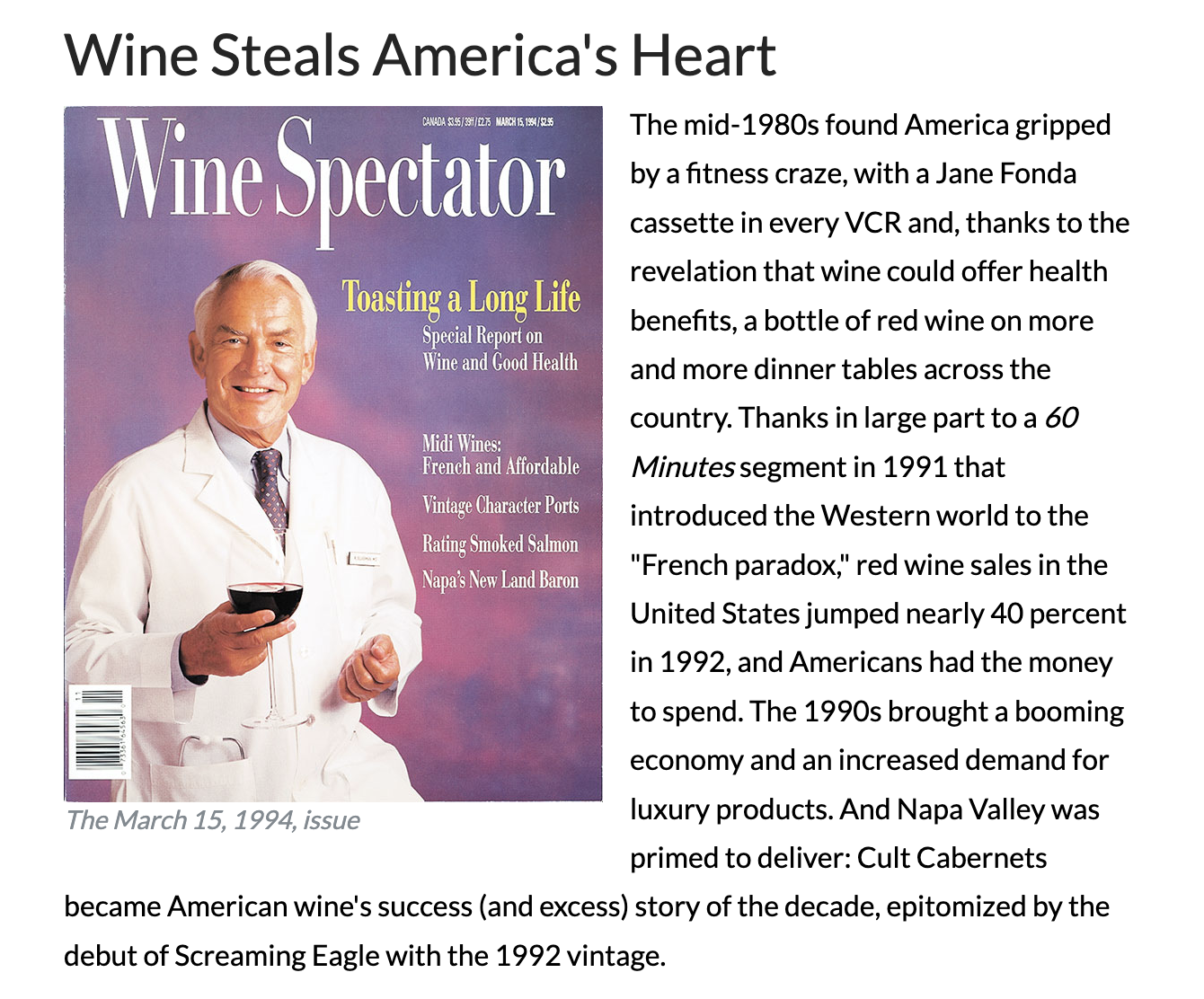
Red wine sales in the US jumped nearly 40% in 1992. The idea that wine was good for your heart became conventional wisdom.

But Wait…

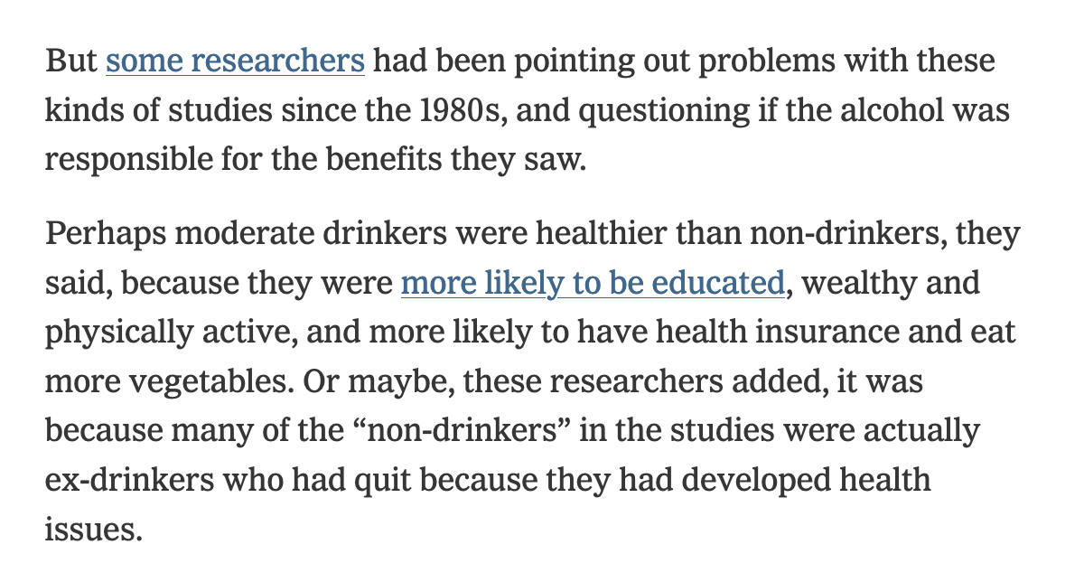
Moderate wine drinkers tend to be more educated, wealthier, more physically active, and more likely to have health insurance.

And many “non-drinkers” were actually ex-drinkers who had quit because of health problems.

In DAG terms: What kinds of bias are these?

Better Methods, Different Answers

Using Mendelian randomization — genetic variants as instruments — alcohol at all levels was associated with increased cardiovascular risk.

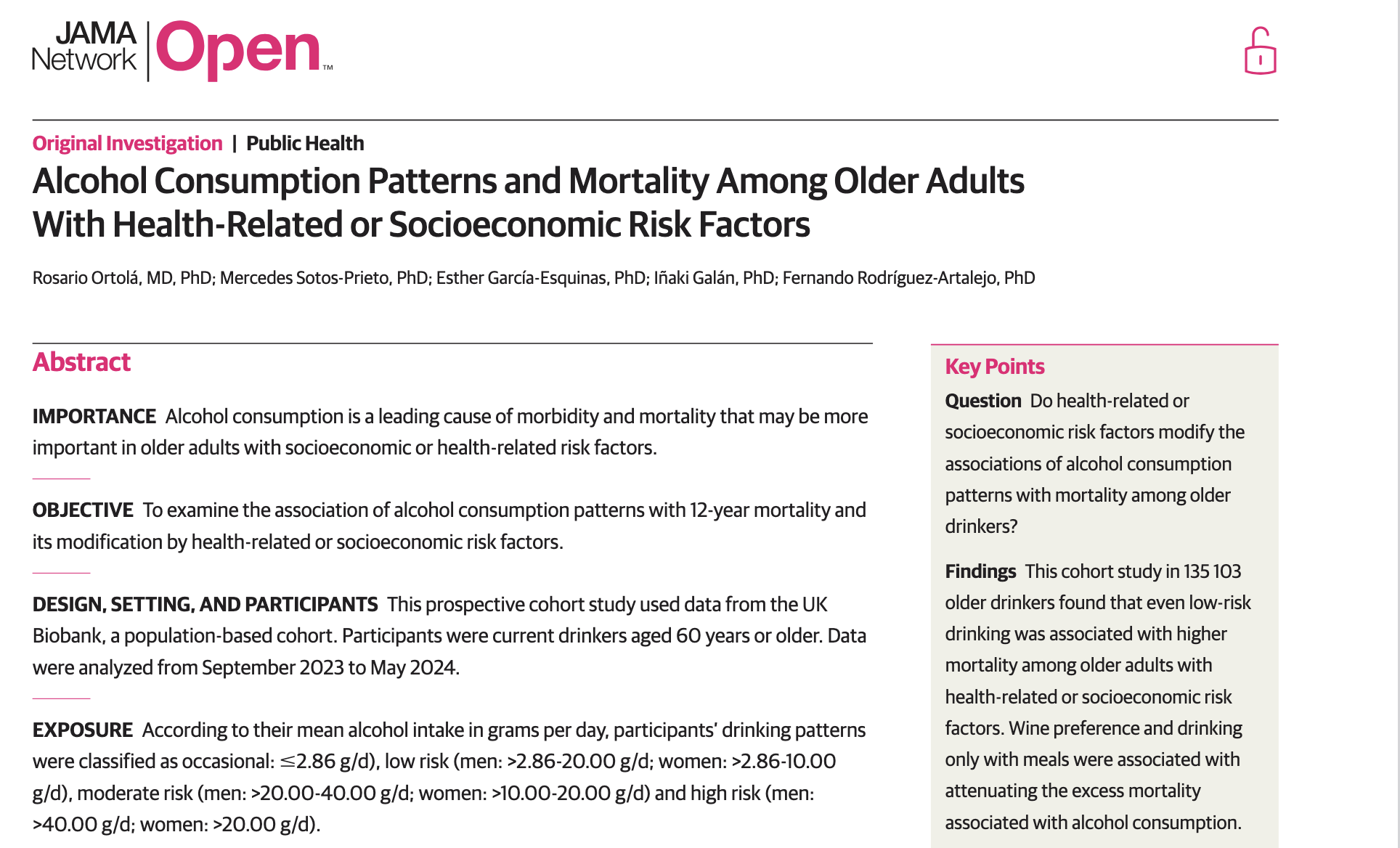
Even among “low-risk” drinkers, alcohol was associated with higher mortality when accounting for health and SES risk factors.

Your Turn: Wine and Health Worksheet

Now apply DAG thinking to this question using the worksheet handout:

List all relevant variables
Draw arrows between them
Simplify your DAG
List all paths from Wine to Heart Health
Determine what to control for

Tip from The Effect

Start with your treatment and outcome. Then ask: “What are all the things that cause my treatment? What are all the things that cause my outcome? Do any of those overlap?” Those overlapping causes are your confounders.

Summary

Key Takeaways

The DGP is what we’re trying to understand. A DAG is our best model of that process.
Association ≠ Causation. DAGs help us think systematically about why.
OVB = an open backdoor path. If a confounder is omitted, the path stays open and your estimate is biased.
The Backdoor Criterion is mechanical. Once you draw the DAG, you can determine what to control for.
Collider bias is real. Controlling for the wrong variable can introduce bias by opening a closed path.
Randomization is powerful. Random assignment closes backdoor paths by design.

What’s Next?

These ideas connect directly to Chapter 9: Assessing Regression Validity:

Omitted variable bias = an open backdoor path you haven’t closed
Measurement error = your DAG nodes don’t match what you actually measured
Simultaneity / reverse causation = the arrows in your DAG might be wrong

The DAG framework gives you a visual language for diagnosing every threat to internal validity.

For the Curious: d-Separation

The backdoor criterion is actually a special case of a more general concept called d-separation.

Two variables are d-separated by \(\mathbf{Z}\) if every path between them is closed after conditioning on \(\mathbf{Z}\)
If d-separated, the variables are conditionally independent given \(\mathbf{Z}\)

You don’t need to know d-separation for this course — the backdoor criterion is the tool you’ll use. But if you want to go deeper, see The Effect Chapter 8 or Pearl (2009).