Nonlinear Relationships

Beyond the Straight Line

ECON3500: Econometrics and Applications

Spring 2026

What You’ll Learn Today

Central Question

What if the relationship between \(X\) and \(Y\) is not a straight line?

By the end of this chapter, you will:

1. Model polynomial relationships (quadratic, cubic)
2. Compute and interpret marginal effects
3. Estimate interaction effects between variables
4. Use logarithmic transformations effectively
5. Apply these tools in Stata

Why Nonlinear?

The Linear Assumption

So far, we’ve assumed relationships are linear:

\[ Y_i = \beta_0 + \beta_1 X_i + u_i \]

Interpretation: A one-unit increase in \(X\) changes \(Y\) by \(\beta_1\) units, regardless of \(X\)’s current value.

But is this realistic?

• Does the first year of education have the same effect as the 20th?
• Does doubling advertising from $1K to $2K have the same effect as doubling from $100K to $200K?
• Does the effect of training depend on whether the worker is already skilled?

The Dose Makes the Poison

Real-World Examples of Nonlinearity

Diminishing returns:

• Fertilizer on crop yield (eventually toxic!)
• Study hours on test scores (exhaustion sets in)
• Experience on wages (plateaus after 30+ years)

Increasing returns:

• Network effects (social media value)
• Learning curves (skills compound)

Interactions:

• Effect of education may depend on ability
• Effect of experience may differ by gender

Three Tools for Nonlinearity

1. Polynomial regression — Add \(X^2\), \(X^3\), etc. to model curvature

2. Interaction terms — Include \(X_1 \cdot X_2\) to allow effects to vary

3. Logarithmic transformations — Use \(\log(Y)\) or \(\log(X)\) for percentage changes

Key Insight

All three remain linear in parameters — we can still use OLS! (A model like \(Y_i = \beta_0 e^{\beta_1 X_i} + u_i\) is not linear in parameters and cannot be estimated by OLS directly.)

The General Nonlinear Regression Model

General Form

\[ Y_i = f(X_{1i}, X_{2i}, \ldots, X_{ki}) + u_i \]

The OLS assumptions carry over unchanged:

1. \(E[u_i \mid X_{1i}, \ldots, X_{ki}] = 0\)
2. \((X_{1i}, \ldots, X_{ki}, Y_i)\) are i.i.d.
3. Large outliers are rare
4. No perfect multicollinearity

Marginal Effects in Nonlinear Models

The effect of a change in \(X_1\), holding \(X_2, \ldots, X_k\) constant:

\[ \Delta Y = f(X_1 + \Delta X_1, X_2, \ldots, X_k) - f(X_1, X_2, \ldots, X_k) \]

Key difference from the linear model: the marginal effect depends on the current value of \(X_1\) (and possibly other variables).

In the linear model: \(\Delta Y = \beta_1 \Delta X_1\) — constant everywhere.

In a nonlinear model: \(\Delta Y\) must be evaluated at a specific value of \(X_1\).

Polynomial Regression

The Quadratic Model

Quadratic Regression Model

\[ Y_i = \beta_0 + \beta_1 X_i + \beta_2 X_i^2 + u_i \]

Why quadratic?

• Allows for curvature in the relationship
• Can capture diminishing or increasing returns
• Flexible, but not too flexible (avoids overfitting)

Still linear in parameters: We estimate \(\beta_0, \beta_1, \beta_2\) via OLS!

Visualizing Quadratic Relationships

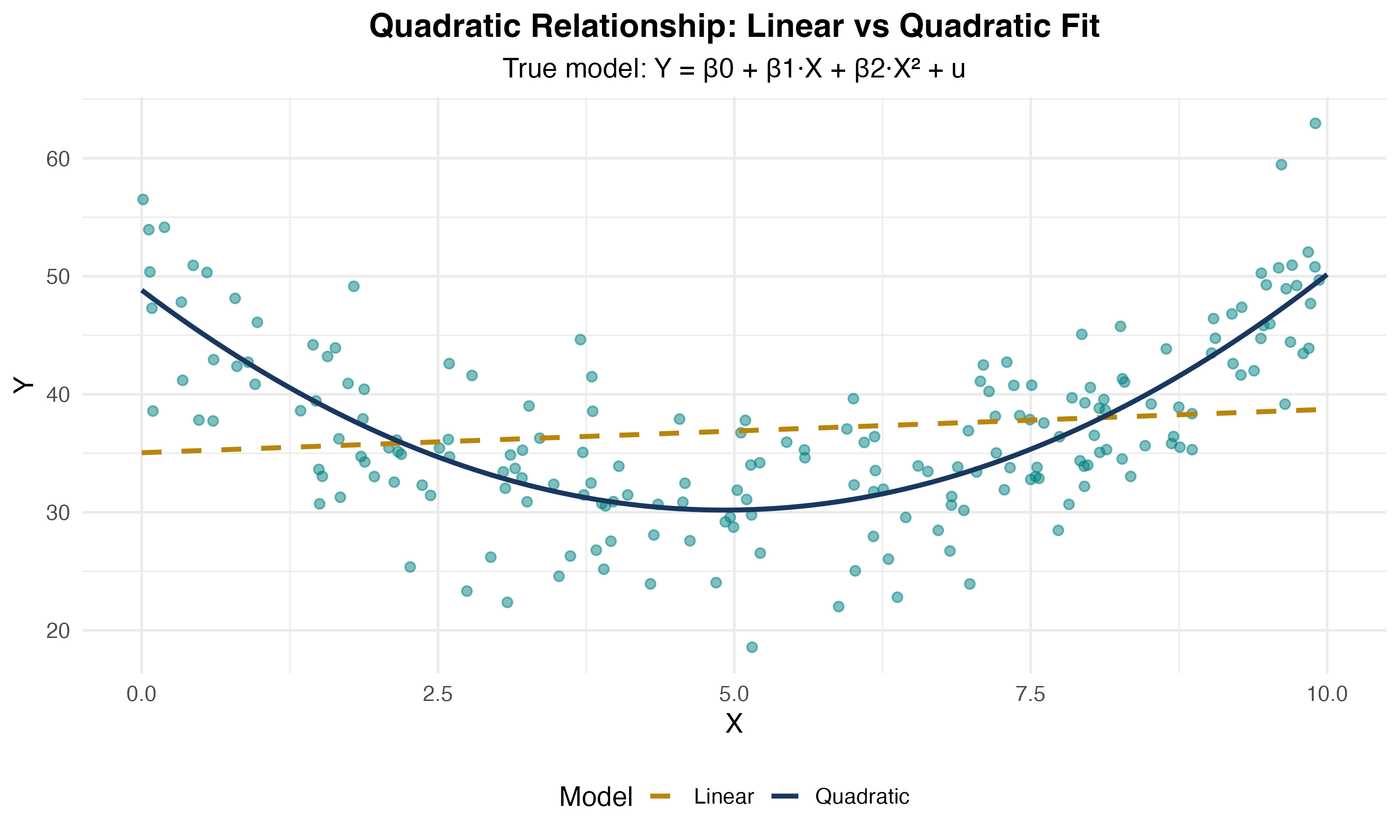
Interpreting Quadratic Coefficients

\[ Y_i = \beta_0 + \beta_1 X_i + \beta_2 X_i^2 + u_i \]

Key point: The effect of \(X\) on \(Y\) is no longer constant!

Marginal Effect in Quadratic Model

\[ \frac{\partial Y}{\partial X} = \beta_1 + 2\beta_2 X \]

The marginal effect depends on the value of \(X\)!

Interpretation:

• At \(X = 0\): marginal effect is \(\beta_1\)
• At \(X = 10\): marginal effect is \(\beta_1 + 20\beta_2\)
• The marginal effect changes by \(2\beta_2\) for each unit increase in \(X\)

Example: Earnings and Experience

Model:

\[ \log(wage) = \beta_0 + \beta_1 \cdot experience + \beta_2 \cdot experience^2 + u \]

Estimated:

\[ \widehat{\log(wage)} = 1.5 + 0.08 \cdot experience - 0.0012 \cdot experience^2 \]

Interpretation:

• \(\hat{\beta}_1 = 0.08 > 0\): wages initially increase with experience
• \(\hat{\beta}_2 = -0.0012 < 0\): inverted-U shape (diminishing returns)
• Marginal effect = \(0.08 - 2(0.0012) \times experience\)

Calculating Marginal Effects

Estimated model:

\[ \log(wage) = 1.5 + 0.08 \cdot exper - 0.0012 \cdot exper^2 \]

At \(exper = 10\) years:

\[ \frac{\partial \log(wage)}{\partial exper} = 0.08 - 2(0.0012)(10) = 0.08 - 0.024 = 0.056 \]

At \(exper = 30\) years:

\[ \frac{\partial \log(wage)}{\partial exper} = 0.08 - 2(0.0012)(30) = 0.08 - 0.072 = 0.008 \]

Interpretation: The wage boost from an additional year of experience falls from 5.6% (at 10 years) to 0.8% (at 30 years).

Finding the Turning Point

For an inverted-U relationship, where does the maximum occur?

Set the marginal effect to zero:

\[ \beta_1 + 2\beta_2 X^* = 0 \quad \Rightarrow \quad X^* = -\frac{\beta_1}{2\beta_2} \]

Example: \(\log(wage) = 1.5 + 0.08 \cdot exper - 0.0012 \cdot exper^2\)

\[ exper^* = -\frac{0.08}{2(-0.0012)} = \frac{0.08}{0.0024} \approx 33.3 \text{ years} \]

Interpretation: Wages peak at about 33 years of experience, then decline.

Visualizing Marginal Effects

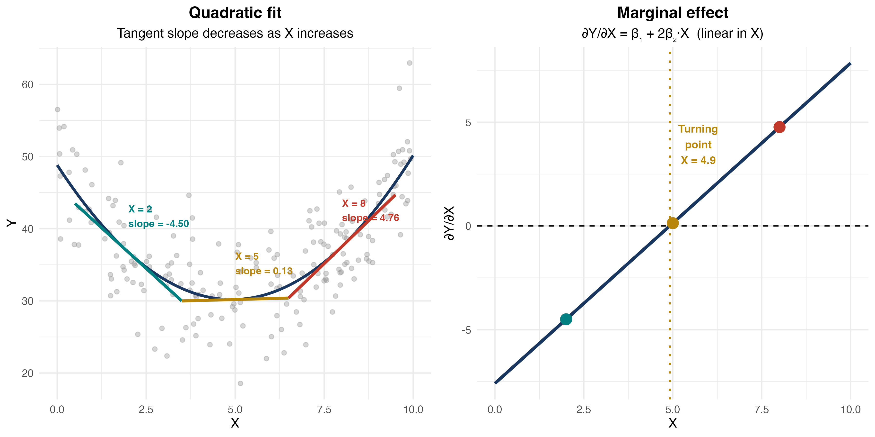
Knowledge Check: Quadratic Model

Question

You estimate: \(sales = 100 + 15 \cdot price - 0.5 \cdot price^2\)

1. What is the marginal effect of price on sales at \(price = 10\)?
2. At what price are sales maximized?

Answer

Part 1: Marginal effect \(= 15 - 2(0.5)(10) = 15 - 10 = 5\). At $10, raising price by $1 increases sales by 5 units.

Part 2: Turning point: \(price^* = -\frac{15}{2(-0.5)} = 15\). Sales are maximized at \(price = 15\).

Cubic and Higher-Order Polynomials

Cubic model:

\[ Y_i = \beta_0 + \beta_1 X_i + \beta_2 X_i^2 + \beta_3 X_i^3 + u_i \]

Marginal effect:

\[ \frac{\partial Y}{\partial X} = \beta_1 + 2\beta_2 X + 3\beta_3 X^2 \]

When to use: Multiple turning points, S-shaped patterns.

Overfitting

Overfitting occurs when we end up fitting the noise in the data rather than the underlying relationship. The model fits the sample well but performs poorly out of sample.

Warning: Higher-order polynomials can overfit and behave erratically at extremes. Use sparingly!

Stata Implementation: Polynomial Regression

Create polynomial terms:

generate experience2 = experience^2
generate experience3 = experience^3

Estimate model:

regress log_wage education experience experience2, robust

Compute marginal effect at mean experience:

summarize experience
scalar exper_mean = r(mean)
display "Marginal effect = " _b[experience] + 2*_b[experience2]*exper_mean

Shortcut using margins:

margins, dydx(experience) at(experience=10)

Testing Whether the Quadratic Term Belongs

Two key hypothesis tests:

Test 1 — Is the quadratic term significant?

\[H_0: \beta_2 = 0 \quad \text{vs.} \quad H_1: \beta_2 \neq 0\]

Use the \(t\)-statistic on \(\hat{\beta}_2\). Reject → evidence of a nonlinear relationship.

Test 2 — Does \(X\) have any effect at all? (joint test)

\[H_0: \beta_1 = \beta_2 = 0\]

Use the \(F\)-statistic. Reject → \(X\) matters (linearly or nonlinearly).

Stata: Testing Polynomial Terms

Test if quadratic term is needed:

regress testscore income income2, robust
test income2

Test if income matters at all (joint F-test):

test income income2

Interpreting the Tests

• Reject \(H_0: \beta_2 = 0\) → keep the quadratic term; relationship is nonlinear
• Fail to reject \(H_0: \beta_2 = 0\) → can simplify back to linear model
• Reject \(H_0: \beta_1 = \beta_2 = 0\) → income has some effect on test scores

Interaction Effects

What Are Interactions?

Interaction Effect

The effect of \(X_1\) on \(Y\) depends on the value of \(X_2\).

Examples:

• Does the effect of job training on employment depend on local unemployment conditions?
• Does the effect of class size on test scores differ by student income level?
• Does the price elasticity of demand differ for necessities vs. luxuries?

Mathematical representation:

\[ Y_i = \beta_0 + \beta_1 X_{1i} + \beta_2 X_{2i} + \beta_3 (X_{1i} \times X_{2i}) + u_i \]

The interaction term is \(X_1 \times X_2\).

Three Types of Interactions

1. Binary × Binary — Does the effect of one group membership vary by another?
   • Example: Does the gender wage gap differ by sector (public vs. private)?
2. Binary × Continuous — Does the slope differ across groups?
   • Example: Does the return to education differ by gender?
3. Continuous × Continuous — Does the effect of one variable depend on the level of another?
   • Example: Does the return to education grow with experience?

All three are estimated the same way: include the product term plus both main effects.

Binary × Binary Interaction

Model:

\[ Y_i = \beta_0 + \beta_1 D_{1i} + \beta_2 D_{2i} + \beta_3 (D_{1i} \cdot D_{2i}) + u_i \]

where \(D_1\) and \(D_2\) are dummy variables.

Predicted values for each group:

	\(D_2 = 0\)	\(D_2 = 1\)
\(D_1 = 0\)	\(\beta_0\)	\(\beta_0 + \beta_2\)
\(D_1 = 1\)	\(\beta_0 + \beta_1\)	\(\beta_0 + \beta_1 + \beta_2 + \beta_3\)

\(\beta_3\) captures the extra effect of being in both groups simultaneously — beyond what you’d expect from the main effects alone.

Example: Gender Gap by Sector

Question: Does the gender wage gap differ in the public sector?

Model:

\[ wage = \beta_0 + \beta_1 \cdot female + \beta_2 \cdot public + \beta_3 (female \times public) + u \]

Estimated:

\[ \hat{wage} = 25 - 4 \cdot female + 3 \cdot public + 2 \cdot (female \times public) \]

What is the predicted wage for each group? What does \(\hat{\beta}_3\) tell us?

Continuous × Continuous Interaction

Model:

\[ Y_i = \beta_0 + \beta_1 X_{1i} + \beta_2 X_{2i} + \beta_3 (X_{1i} \cdot X_{2i}) + u_i \]

Marginal effect of \(X_1\):

\[ \frac{\partial Y}{\partial X_1} = \beta_1 + \beta_3 X_2 \]

Interpretation:

• When \(X_2 = 0\): effect of \(X_1\) is \(\beta_1\)
• When \(X_2 = 10\): effect of \(X_1\) is \(\beta_1 + 10\beta_3\)
• The effect of \(X_1\) changes by \(\beta_3\) for each unit increase in \(X_2\)

Example: Education and Experience Interaction

Question: Does the return to education depend on experience?

Model:

\[ wage = \beta_0 + \beta_1 \cdot education + \beta_2 \cdot experience + \beta_3 (education \times experience) + u \]

Estimated:

\[ \hat{wage} = 2.0 + 1.5 \cdot education + 0.3 \cdot experience + 0.05 \cdot (education \times experience) \]

Interpretation:

• For someone with 0 years experience: return to education = $1.50/year
• For someone with 10 years experience: return = $1.50 + 0.05(10) = $2.00/year
• Education becomes more valuable as you gain experience!

Visualizing Continuous × Continuous Interactions

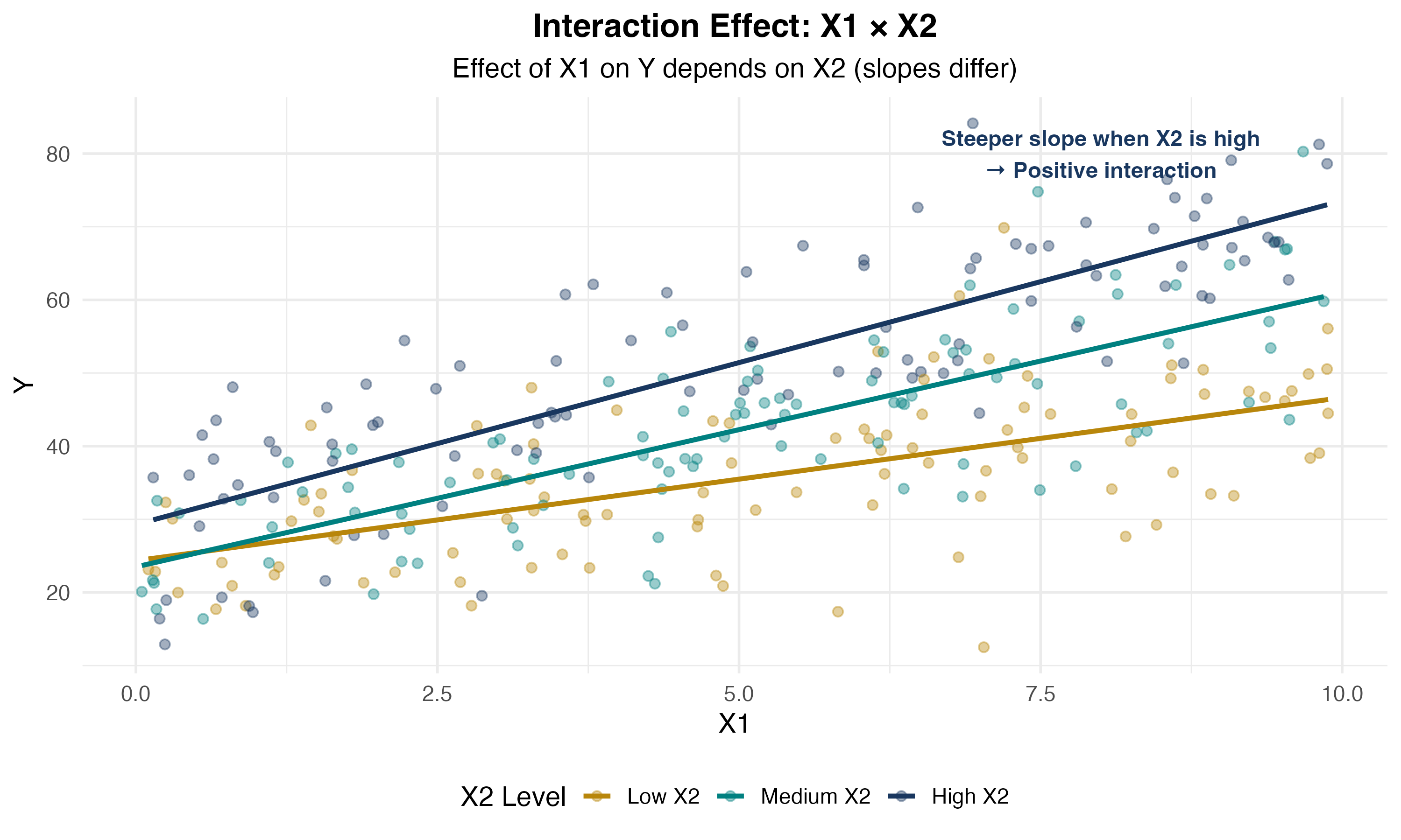
Binary × Continuous Interaction

Model:

\[ Y_i = \beta_0 + \beta_1 X_i + \beta_2 D_i + \beta_3 (X_i \cdot D_i) + u_i \]

where \(D_i\) is a dummy variable (0 or 1).

Interpretation:

• When \(D = 0\): \(Y = \beta_0 + \beta_1 X\) (baseline group)
• When \(D = 1\): \(Y = (\beta_0 + \beta_2) + (\beta_1 + \beta_3) X\) (treatment group)
• \(\beta_2\): intercept shift | \(\beta_3\): slope shift

Example: Gender Wage Gap

Model:

\[ wage = \beta_0 + \beta_1 \cdot education + \beta_2 \cdot female + \beta_3 (education \times female) + u \]

Estimated:

\[ \hat{wage} = 3.0 + 2.0 \cdot education - 1.5 \cdot female - 0.3 \cdot (education \times female) \]

Interpretation:

• Men (\(female = 0\)): \(wage = 3.0 + 2.0 \cdot education\)
• Women (\(female = 1\)): \(wage = 1.5 + 1.7 \cdot education\)
• Women earn $1.50 less at 0 education; $0.30 less per year of education. Gap widens with education!

Visualizing Binary × Continuous Interactions

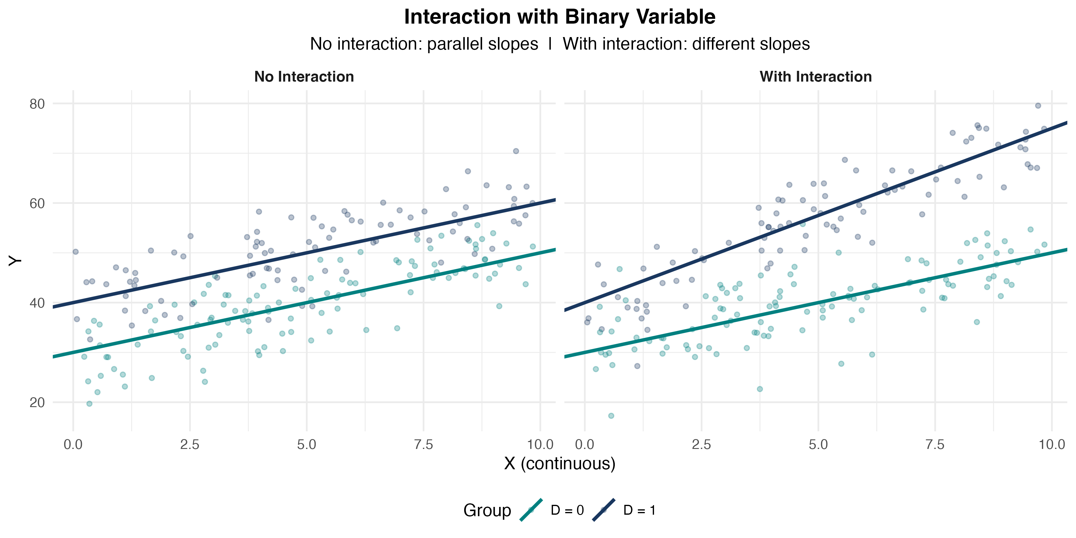
Knowledge Check: Interaction Effects

Question

You estimate: \(price = 50 + 10 \cdot quality + 5 \cdot advertising + 2 \cdot (quality \times advertising)\)

1. What is the marginal effect of advertising when quality = 5?
2. What is the marginal effect of advertising when quality = 10?

Answer

Marginal effect of advertising = \(5 + 2 \times quality\)

Part 1: At quality = 5: effect = \(5 + 2(5) = 15\)

Part 2: At quality = 10: effect = \(5 + 2(10) = 25\)

Advertising is more effective for higher-quality products!

Stata Implementation: Interactions

Method 1: Create interaction manually

generate educ_exper = education * experience
regress wage education experience educ_exper, robust

Method 2: Factor variable notation (preferred)

regress wage c.education##c.experience, robust // continuous × continuous
regress wage c.education##i.female, robust // continuous × dummy
regress wage i.female##i.public, robust // dummy × dummy

Compute marginal effects at different values:

margins, dydx(education) at(experience=(0 10 20 30))

Factor variable prefixes

• c.varname — tells Stata to treat the variable as continuous
• i.varname — tells Stata to treat the variable as categorical/dummy
• ## — includes the interaction and both main effects automatically

String variables: Factor notation requires numeric variables. If your variable is a string, convert it first: encode strvar, gen(numvar), then use i.numvar. Alternatively, use the older xi: prefix: xi: regress wage i.female*education.

Common Mistakes with Interactions

Mistake 1: Including interaction but omitting main effects

Never include \(X_1 \times X_2\) without also including \(X_1\) and \(X_2\) separately. Omitting a main effect forces a constraint (e.g., that the baseline group has a zero intercept) that is almost always wrong.

Mistake 2: Interpreting \(\beta_1\) as “the” effect of \(X_1\)

In \(Y = \beta_0 + \beta_1 X_1 + \beta_2 X_2 + \beta_3 X_1 X_2\), the effect of \(X_1\) is \(\beta_1 + \beta_3 X_2\) — it depends on \(X_2\). \(\beta_1\) is only the effect of \(X_1\) when \(X_2 = 0\), which may not be a meaningful value.

Mistake 3: Testing the wrong hypothesis

To test whether an interaction matters, test \(H_0: \beta_3 = 0\) (not \(H_0: \beta_1 = 0\)). In Stata: test after regress, or read the \(t\)-statistic on the interaction term directly.

Choosing Interaction Terms

When should you include an interaction?

1. Theory first — Is there a compelling reason that the effect of \(X_1\) depends on \(X_2\)? If yes, include the interaction regardless of significance.

2. Statistical test — Test \(H_0: \beta_3 = 0\). If rejected, the interaction is statistically significant.

3. Model fit — The adjusted \(R^2\) (\(\bar{R}^2\)) penalizes for added parameters. If \(\bar{R}^2\) rises when you add the interaction term, that provides additional support for including it.

Logarithmic Specifications

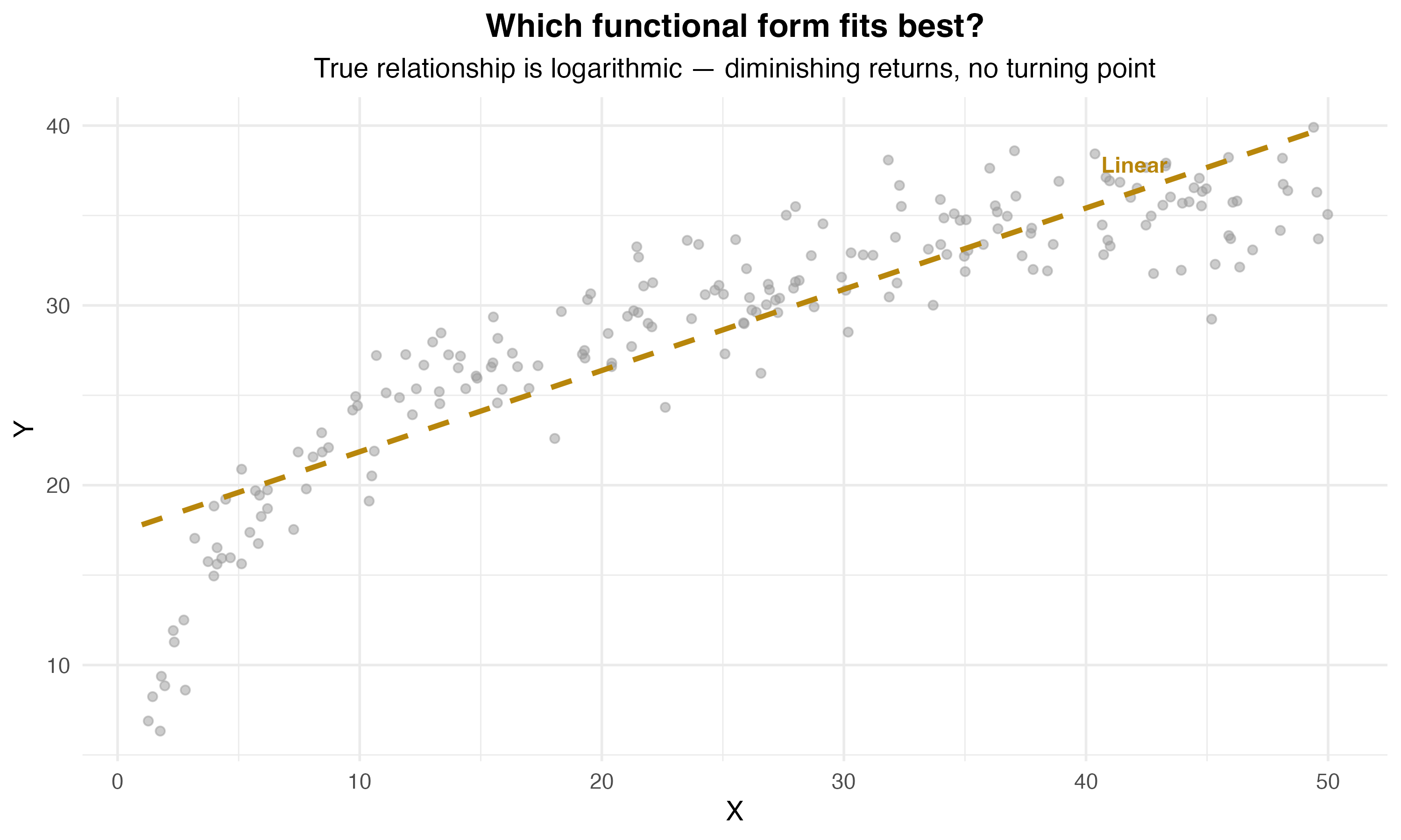
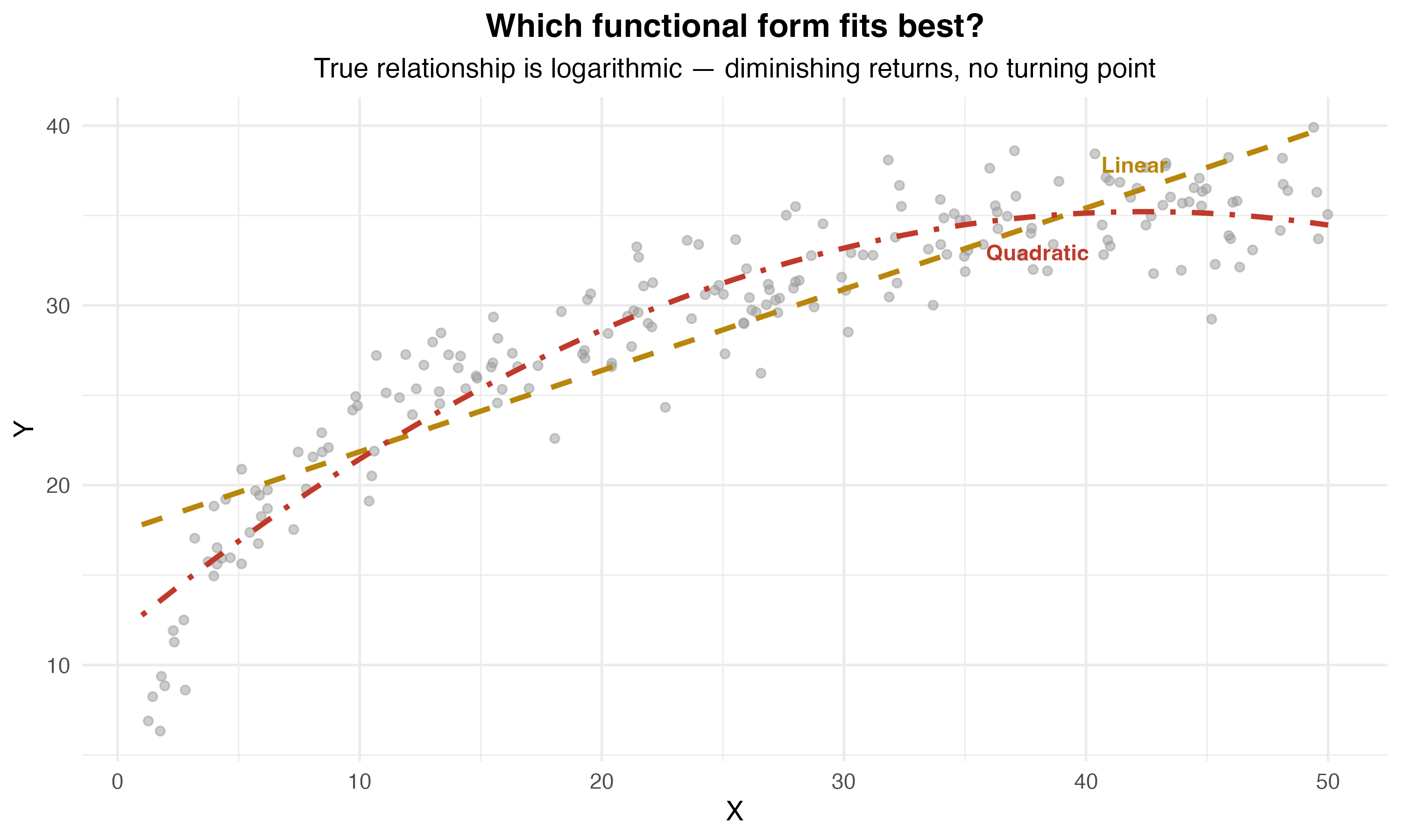
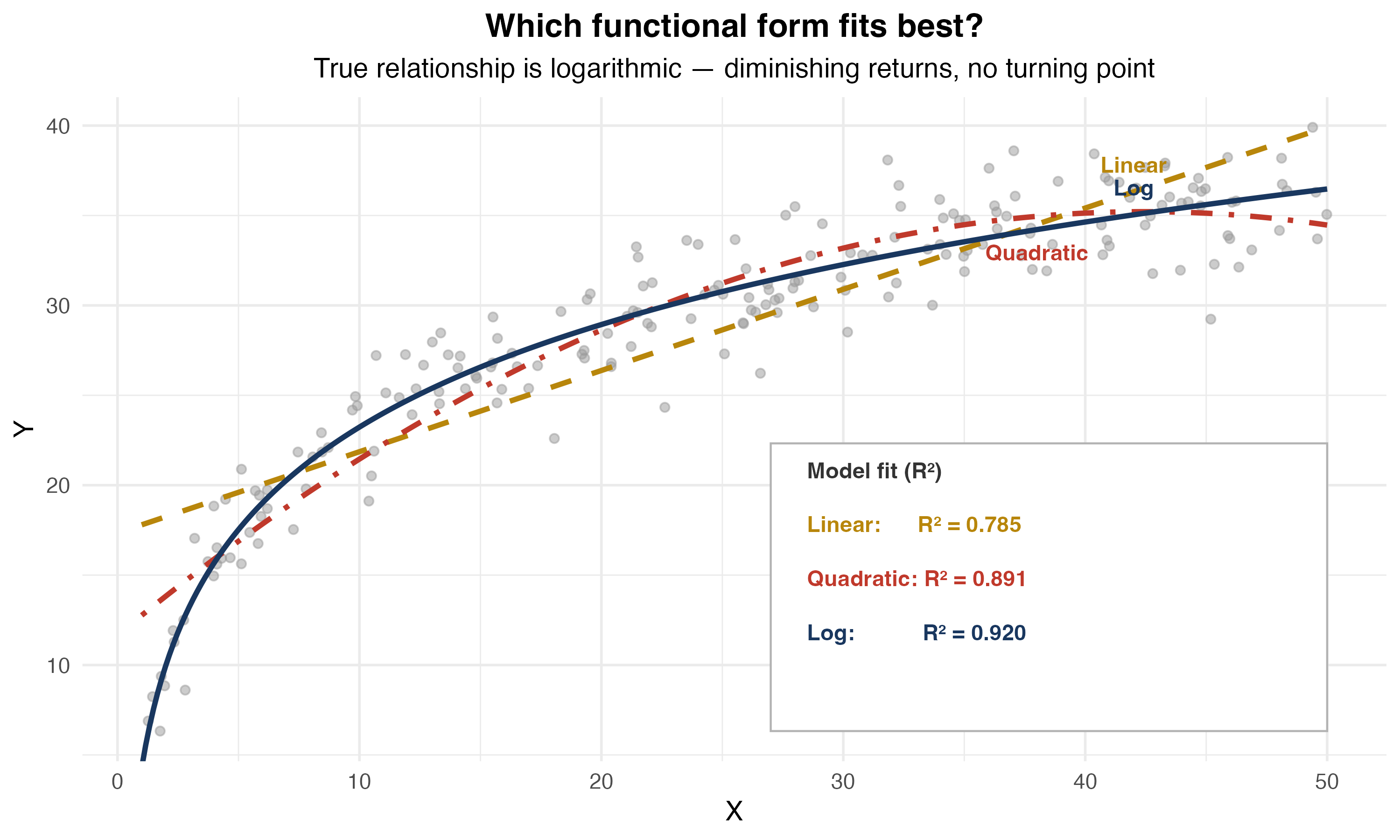
When Is a Log the Right Tool?

Why Logarithms?

Three key advantages:

1. Percentage interpretation — Coefficients represent percentage changes, not unit changes
2. Diminishing returns automatically — \(\log(X)\) is concave (built-in curvature!)
3. Elasticities — Direct estimates of elasticity in log-log models

Important: Can only take log of positive variables!

Advantages and Caveats of Logs

Advantages:

• Coefficients have convenient percentage/elasticity interpretations
• Slope coefficients are invariant to rescaling of the variable
• Often reduces the influence of outliers
• Can improve normality and homoskedasticity of residuals

Caveats:

• Cannot log zero or negative values (income, price: fine; test scores starting at 0: not fine)
• Do not log variables measured in years or percentage points (e.g., age, interest rate)
• Harder to reverse the log transformation when constructing predictions

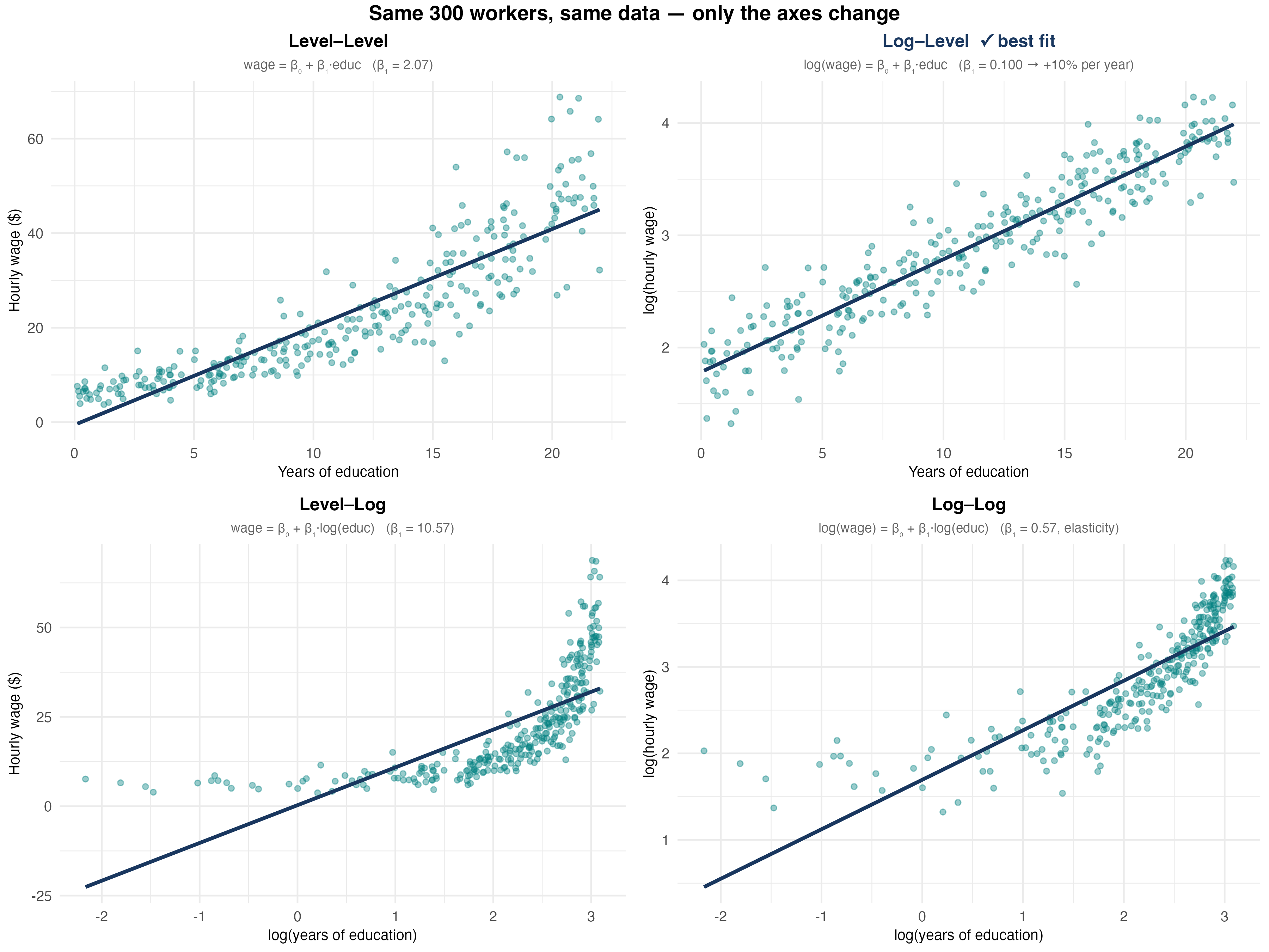
Four Logarithmic Models

Model	Equation	Interpretation
Level-level	\(Y = \beta_0 + \beta_1 X\)	\(\Delta Y = \beta_1 \Delta X\)
Log-level	\(\log Y = \beta_0 + \beta_1 X\)	\(\%\Delta Y = 100\beta_1 \Delta X\)
Level-log	\(Y = \beta_0 + \beta_1 \log X\)	\(\Delta Y = (\beta_1/100) \%\Delta X\)
Log-log	\(\log Y = \beta_0 + \beta_1 \log X\)	\(\%\Delta Y = \beta_1 \%\Delta X\)

Key insight: Each log transforms a unit change into a percentage change!

The Log Approximation

Key Fact

For small changes in \(X\):

\[100 \cdot \Delta \log(X) \approx \%\Delta X\]

Change in \(X\)	Log approximation	Exact % change
50 → 51	1.98%	2.00%
50 → 50.5	0.995%	1.00%
50 → 60	18.2%	20.0%
50 → 80	47.0%	60.0%

Rule of thumb: Approximation works well for changes up to ~10%. For larger changes, use the exact formula: \(\%\Delta Y = 100(e^{\hat{\beta}} - 1)\).

Level-Level (Baseline)

\[ Y_i = \beta_0 + \beta_1 X_i + u_i \]

Interpretation: A one-unit increase in \(X\) is associated with a \(\beta_1\)-unit change in \(Y\).

Example: \(wage = 5 + 2.5 \cdot education\) — Each additional year of education increases wages by $2.50/hour.

Log-Level

\[ \log(Y_i) = \beta_0 + \beta_1 X_i + u_i \]

Log-Level Interpretation

A one-unit increase in \(X\) is associated with a \(100\beta_1\)% change in \(Y\).

Example: \(\log(wage) = 1.5 + 0.08 \cdot education\) — Each additional year of education increases wages by 8%.

Large changes: When \(100\beta_1 > 10\%\), use the exact formula:

\[\%\Delta \hat{Y} = 100(e^{\hat{\beta}_1} - 1)\]

Always preserve the sign of the coefficient!

Level-Log

\[ Y_i = \beta_0 + \beta_1 \log(X_i) + u_i \]

Level-Log Interpretation

A 1% increase in \(X\) is associated with a \(\beta_1/100\) unit change in \(Y\).

Example: \(wage = 2 + 5 \log(experience)\) — A 1% increase in experience increases wages by $0.05/hour. Doubling experience (100% increase) raises wages by $5/hour.

Where Does Log-Level Come From?

Model: \(\log(wage) = \beta_0 + \beta_1 \cdot educ + u\)

Goal: What happens to \(wage\) when \(educ\) increases by 1?

Step 1: Take the partial derivative of both sides with respect to \(educ\):

\[\Delta \log(wage) = \beta_1 \cdot \Delta educ\]

Step 2: Multiply both sides by 100:

\[100 \cdot \Delta \log(wage) = 100\beta_1 \cdot \Delta educ\]

Step 3: Apply the log approximation (\(100 \cdot \Delta \log(x) \approx \%\Delta x\)):

\[\%\Delta wage \approx 100\beta_1 \cdot \Delta educ\]

Conclusion: A one-unit increase in \(educ\) is associated with a \(100\beta_1\)% change in \(wage\).

Where Does Level-Log Come From?

Model: \(wage = \beta_0 + \beta_1 \log(educ) + u\)

Goal: What happens to \(wage\) when \(educ\) increases by 1%?

Step 1: Take the partial derivative of both sides with respect to \(\log(educ)\):

\[\Delta wage = \beta_1 \cdot \Delta \log(educ)\]

Step 2: Multiply and divide the right side by 100:

\[\Delta wage = \frac{\beta_1}{100} \cdot 100 \cdot \Delta \log(educ)\]

Step 3: Apply the log approximation (\(100 \cdot \Delta \log(x) \approx \%\Delta x\)):

\[\Delta wage \approx \frac{\beta_1}{100} \cdot \%\Delta educ\]

Conclusion: A 1% increase in \(educ\) is associated with a \(\beta_1 / 100\) unit change in \(wage\).

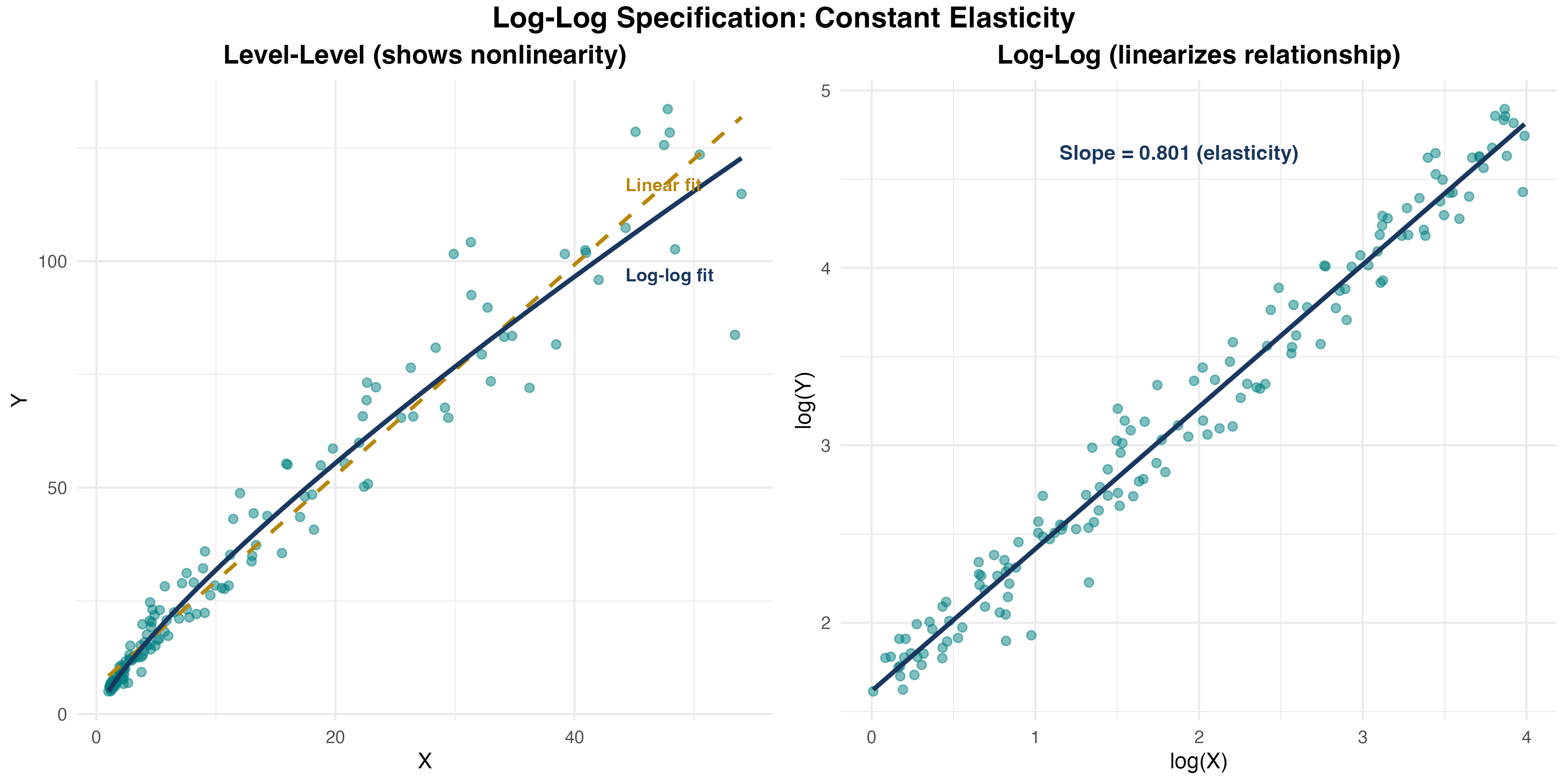
Log-Log (Elasticity)

\[ \log(Y_i) = \beta_0 + \beta_1 \log(X_i) + u_i \]

Log-Log Interpretation

\(\beta_1\) is the elasticity of \(Y\) with respect to \(X\). A 1% increase in \(X\) leads to a \(\beta_1\)% change in \(Y\).

Example: \(\log(quantity) = 2.5 - 1.2 \log(price)\) — A 1% increase in price leads to a 1.2% decrease in quantity (price elasticity of demand).

Visualizing Log Specifications

Log-Log Specification in Detail

Knowledge Check: Log Specifications

What are the units? How do we interpret each coefficient?

• 1. \(wage = 5 + 0.3 \cdot experience\)
• 2. \(\log(wage) = 1.2 + 0.04 \cdot experience\)
• 3. \(wage = 8 + 2.5 \log(experience)\)
• 4. \(\log(wage) = 1.5 + 0.15 \log(experience)\)

Knowledge Check: Answers

a) \(wage = 5 + 0.3 \cdot experience\) — level-level \(\Delta wage = 0.3 \cdot \Delta experience\) → each additional year raises wages by $0.30

b) \(\log(wage) = 1.2 + 0.04 \cdot experience\) — log-level \(\Delta \log(wage) = 0.04 \cdot \Delta experience\), so \(\%\Delta wage \approx 100(0.04)(1)\) → each additional year raises wages by 4%

c) \(wage = 8 + 2.5 \log(experience)\) — level-log \(\Delta wage = 2.5 \cdot \Delta \log(experience)\), so \(\Delta wage = (2.5/100) \cdot \%\Delta experience\) → a 1% increase in experience raises wages by $0.025

d) \(\log(wage) = 1.5 + 0.15 \log(experience)\) — log-log (elasticity) \(\%\Delta wage = 0.15 \cdot \%\Delta experience\) → a 1% increase in experience raises wages by 0.15%

Interpretation Guide Summary

Model	Specification	Interpret \(\hat\beta_1\) as…
Level–Level	\(Y = \beta_0 + \beta_1 X\)	+1 unit in \(X\) → \(+\beta_1\) units in \(Y\)
Log–Level	\(\log(Y) = \beta_0 + \beta_1 X\)	+1 unit in \(X\) → \(+(100\beta_1)\)% in \(Y\)
Level–Log	\(Y = \beta_0 + \beta_1 \log(X)\)	+1% in \(X\) → \(+\beta_1/100\) units in \(Y\)
Log–Log	\(\log(Y) = \beta_0 + \beta_1 \log(X)\)	+1% in \(X\) → \(+\beta_1\)% in \(Y\) (elasticity)

Memory aid

• Is \(Y\) logged? → interpret as % change in \(Y\)
• Is \(X\) logged? → interpret as % change in \(X\)
• Both logged? → elasticity

Stata Implementation: Logs

Generate log variables:

generate log_wage = log(wage)
generate log_sales = log(sales)
generate log_price = log(price)

Estimate different specifications:

* Log-level
regress log_wage education experience, robust

* Level-log
regress wage log_experience log_sales, robust

* Log-log
regress log_quantity log_price log_income, robust

Important: Always use natural log (log in Stata), not log10 or log2!

When to Use Logarithms?

Ask: which is more meaningful for your variable?

1. Absolute changes → use levels
   • “An additional year of education raises wages by $3”
2. Percent changes → use logs
   • “An additional year of education raises wages by 8%”

Practical Guidance

• Wages, income, prices, GDP → usually log (wide range; percent interpretation natural)
• Test scores, years of education, rates → usually levels (bounded; percentage interpretation less natural)
• Variables that can be zero or negative → cannot log; use levels
• You do not need to transform all variables — mix levels and logs as theory dictates

Bringing It All Together

The Nonlinear Toolkit

Tool	Use When	Gives You
Polynomial	Curved relationships, turning points	Marginal effects that vary with \(X\)
Interactions	Effect depends on another variable	Different slopes for different groups
Logarithms	Wide ranges, percentage interpretation	Elasticities, diminishing returns

Key principle: All remain linear in parameters — we can use OLS and all our inference tools!

Key Formulas Summary

Model	Marginal Effect
Quadratic	\(\frac{\partial Y}{\partial X} = \beta_1 + 2\beta_2 X\)
Interaction	\(\frac{\partial Y}{\partial X_1} = \beta_1 + \beta_3 X_2\)
Log-level	\(\frac{\%\Delta Y}{\Delta X} = 100\beta_1\)
Level-log	\(\frac{\Delta Y}{\%\Delta X} = \beta_1/100\)
Log-log (elasticity)	\(\frac{\%\Delta Y}{\%\Delta X} = \beta_1\)

Turning point: \(X^* = -\frac{\beta_1}{2\beta_2}\) (quadratic model)