Hypothesis Tests and Confidence Intervals in Multiple Regression

SW Chapter 7

ECON3500: Econometrics and Applications

Spring 2026

Learning Objectives

  1. Construct and interpret confidence intervals for individual coefficients in multiple regression
  2. Test hypotheses about one coefficient (review from Ch5)
  3. Test hypotheses about one restriction involving multiple coefficients
  4. Construct and interpret joint hypothesis tests (the F-test)
  5. Explain why testing coefficients one at a time can be misleading

Three Types of Hypothesis Tests

A Taxonomy of Tests

Type Null Hypothesis Example Statistic
1. One restriction, one coefficient \(H_0: \beta_j = \beta_{j,0}\) \(H_0: \beta_1 = 0\) \(t\)
2. One restriction, multiple coefficients \(H_0: \beta_j = \beta_m\) \(H_0: \beta_1 = \beta_2\) \(t\)
3. Multiple restrictions (joint test) \(H_0: \beta_j = \beta_{j,0}, \; \beta_m = \beta_{m,0}, \ldots\) \(H_0: \beta_1 = \beta_2 = 0\) \(F\)

Confidence Intervals in Multiple Regression

Confidence Intervals for Individual Coefficients

In simple regression (Ch5), we constructed CIs for \(\beta_1\). The same logic extends to any coefficient in a multiple regression:

\[ \hat{\beta}_j \pm c_{\alpha/2} \cdot SE(\hat{\beta}_j) \]

where \(c_{\alpha/2}\) is the critical value from the standard normal (large \(n\)):

Confidence Level \(c_{\alpha/2}\)
90% 1.645
95% 1.96
99% 2.58

Interpretation

In 95% of possible samples that might be drawn, the confidence interval will contain the true value of \(\beta_j\).”

Side Note: What CIs Are and Are Not

CIs are NOT:

  • The probability that the parameter is in the interval
  • Our confidence we have the right answer
  • A statement about the parameter after we observe it

CIs ARE:

  • Constructed using a procedure that works 95% of the time
  • Frequentist: the interval contains the true parameter in 95% of repeated samples
  • Before sampling, our procedure has 95% coverage

In sum: - Before sampling: Our procedure has 95% coverage probability - After sampling: The interval either contains the parameter or it doesn’t

There’s a 95% chance that a CI contains the true parameter, but not that the estimated CI contains the true parameter.

CIs in Multiple Regression: What Changes?

Compared to simple regression:

  • The formula is the same: \(\hat{\beta}_j \pm c \cdot SE(\hat{\beta}_j)\)
  • The standard errors change because they now account for correlations among regressors

Key insight: Adding control variables can either increase or decrease the SE of \(\hat{\beta}_j\):

  • Reduces SE if the added variable explains variation in \(Y\) (reduces \(\hat{\sigma}^2_u\))
  • Increases SE if the added variable is correlated with \(X_j\) (multicollinearity)

1. One Restriction, One Coefficient: \(\beta_j = \beta_{j,0}\)

  1. Select your significance level (\(\alpha = 0.01\))

  2. State your null hypothesis:

    • \(H_0: \beta_j = \beta_{j,0}\)
    • \(H_a: \beta_j \neq \beta_{j,0}\)
  3. Compute the t-statistic: \[t = \frac{\hat{\beta_j}-\beta_{j,0}}{SE(\hat{\beta_j})}\]

  4. Compare the t-statistic to your critical value (2.58) and reject null if \(|t|>c\)

  5. (Optional) Construct your confidence interval: \[\left(\hat{\beta_j} - 2.58 \cdot SE(\hat{\beta_j}), \hat{\beta_j}+2.58 \cdot SE(\hat{\beta_j})\right)\]

2. One Restriction, Two Coefficients: \(\beta_j = \beta_m\)

  1. Select your significance level (\(\alpha = 0.01\))

  2. State your null hypothesis: \(H_0: \beta_1 = \beta_2\) vs \(H_a: \beta_1 \neq \beta_2\)

  3. Transform your regression: \[\begin{align} y_i &= \beta_0 + \beta_1x_{1i} + \beta_2x_{2i} + u_i\\ y_i &= \beta_0 + \beta_1x_{1i} + \beta_2x_{1i} - \beta_2x_{1i}+ \beta_2x_{2i} + u_i\\ y_i &= \beta_0 + (\beta_1- \beta_2)x_{1i} + \beta_2(x_{1i} + x_{2i}) + u_i\\ y_i &= \beta_0 + \gamma_1x_{1i} + \beta_2w_{i}+ u_i \end{align}\]

    and instead test \(H_0: \gamma_1 = 0\) vs. \(H_1: \gamma_1 \neq 0\)

  4. Repeat remaining steps

3. Multiple Restrictions (Under Homoskedasticity)

There are lots of variants, but this is the one we will compute by hand

  1. Select your significance level (\(\alpha = 0.01\))

  2. State your null hypothesis: \(H_0: \beta_1 = \beta_2 = \beta_3\) vs any part not true

  3. Estimate model with variables you are testing (unrestricted) and without (restricted)

  4. Calculate \(F\)-statistic \[F = \frac{(SSR_r - SSR_{ur})/q}{SSR_{ur}/(n-k_{ur}-1)} = \frac{(R^2_{ur} - R^2_{r})/q}{(1-R^2_{ur})/(n-k_{ur}-1)} \sim F_{q,n-k_{ur}-1}\]

  5. Compare the F-statistic to your critical value from a \(F_{q,n-k_{ur}-1}\) distribution and reject null if \(F>c\) (usually from \(F_{q,\infty}\) distribution)

Extendedxample: The STAR Experiment

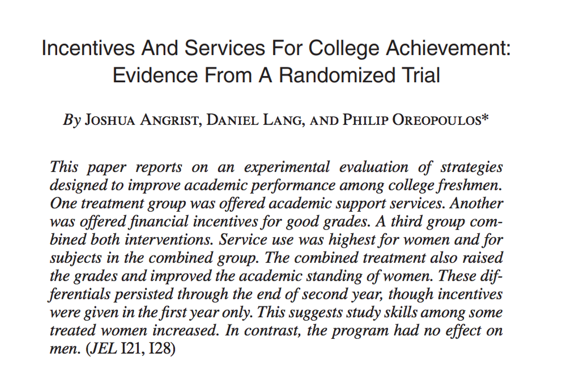
Angrist, Lang, and Oreopoulos (2009)

We’re going to think about predictors of year 1 college GPA.

The STAR Experiment: Context

Setting: A satellite campus of a large Canadian university (University of Toronto at Scarborough)

Research question: Can academic support services and financial incentives improve first-year academic performance?

Three treatment groups (randomly assigned):

  • SSP (Student Support Program): peer advising and facilitated study groups
  • SFP (Student Fellowship Program): merit-based scholarships for meeting GPA targets
  • SFSP: combined SSP + SFP treatment

Key findings: The combined program (SFSP) improved grades for women, particularly those with weaker high school backgrounds. Support services alone or financial incentives alone had limited effects.

Our focus today: We’ll use the control variables from this study — gender, mother tongue, and high school quartile — to practice hypothesis testing. This is about the predictors of Year 1 GPA, not the treatment effects.

Recall: The Dummy Variable Trap (Ch6)

When including a categorical variable with \(m\) categories, include \(m - 1\) dummy variables and leave one as the reference group.

In our example:

  • Mother tongue has 3 categories: English, French, Other
  • We include mt_french and mt_other; English is the excluded reference group
  • Coefficients on mt_french and mt_other are interpreted relative to English speakers

Quick Check

If we included all three dummies plus an intercept, what would happen?

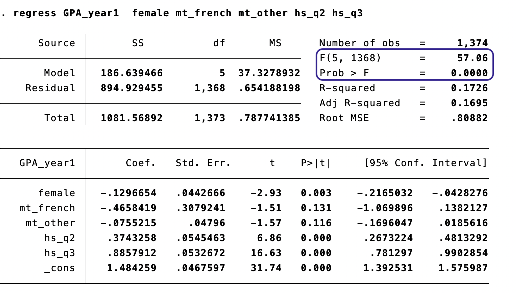
The Base Regression

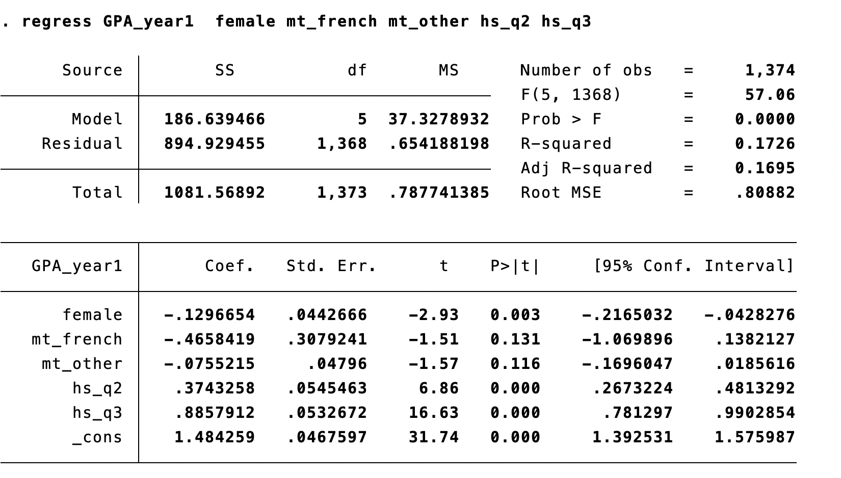
regress GPA_year1 female mt_french mt_other hs_q2 hs_q3, robust

Controls for gender, mother tongue, and HS quartile (no top quartile!)

Choice of Excluded Group Only Affects Interpretation

English mother tongue excluded: \[\widehat{GPAyear1}= 1.484 - 0.130 \cdot female - 0.466 \cdot mt_{french} - 0.076 \cdot mt_{other} + 0.374 \cdot hs_{q2} + 0.886 \cdot hs_{q3}\]

“Other” mother tongue excluded: \[\widehat{GPAyear1}= 1.409 - 0.130 \cdot female - 0.076 \cdot mt_{english} - 0.390 \cdot mt_{french} + 0.374 \cdot hs_{q2} + 0.886 \cdot hs_{q3}\]

Choice of Excluded Group Only Affects Interpretation

For simplicity, assume \(female = 0\), \(hs_{q2} = 0\), and \(hs_{q3} = 0\)

English mother tongue excluded: \[\widehat{GPAyear1}= 1.484 - 0.130 \cdot female - 0.466 \cdot mt_{french} - 0.0755 \cdot mt_{other} + 0.374 \cdot hs_{q2} + 0.886 \cdot hs_{q3}\]

\[\begin{align} E[GPAyear1 | mt_{english} = 1] &= 1.484\\ E[GPAyear1 | mt_{french} = 1] &= 1.484 - 0.466 = 1.018\\ E[GPAyear1 | mt_{other} = 1] &= 1.4843 - 0.0755 = 1.409 \end{align}\]

Choice of Excluded Group Only Affects Interpretation (cont.)

For simplicity, assume \(female = 0\), \(hs_{q2} = 0\), and \(hs_{q3} = 0\)

“Other” mother tongue excluded: \[\widehat{GPAyear1}= 1.409 - 0.130 \cdot female + 0.0755 \cdot mt_{english} - 0.390 \cdot mt_{french} + 0.374 \cdot hs_{q2} + 0.886 \cdot hs_{q3}\]

\[\begin{align} E[GPAyear1 | mt_{english} = 1] &= 1.4087 + 0.0755 = 1.484\\ E[GPAyear1 | mt_{french} = 1] &= 1.4087 - 0.3903 = 1.018\\ E[GPAyear1 | mt_{other} = 1] &= 1.4087 = 1.409 \end{align}\]

Questions We Could Want to Answer

  • Do French speakers have the same GPA as English speakers? → Type 1: test \(\beta_{french} = 0\)]
  • Do “Other” speakers have the same GPA as English speakers? → Type 1: test \(\beta_{other} = 0\)
  • Do French speakers have the same GPA as “Other” speakers?Type 2
  • Are there any differences in GPA by mother tongue?Type 3

Testing Equality of Two Coefficients

Do French speakers have the same GPA as “Other” speakers?

Population model: \[GPA_i = \beta_0 + \beta_1 \cdot mt_{french} + \beta_2 \cdot mt_{other} + \beta_3 \cdot hs_{q2} + \beta_4 \cdot hs_{q3} + u_i\]

\[H_0: \beta_1 = \beta_2 \quad \text{vs.} \quad H_a: \beta_1 \neq \beta_2\]

Equivalently: \(H_0: \beta_1 - \beta_2 = 0\)

Problem: We can’t directly test this with a standard \(t\)-test on a single coefficient.

Solution: Transform the regression.

The Transformation Trick

Start with: \[y_i = \beta_0 + \beta_1 x_{1i} + \beta_2 x_{2i} + \cdots + u_i\]

Add and subtract \(\beta_2 x_{1i}\): \[y_i = \beta_0 + \beta_1 x_{1i} {\color{teal}{+ \beta_2 x_{1i} - \beta_2 x_{1i}}} + \beta_2 x_{2i} + \cdots + u_i\]

Rearrange: \[y_i = \beta_0 + \underbrace{(\beta_1 - \beta_2)}_{\gamma_1} x_{1i} + \beta_2 \underbrace{(x_{1i} + x_{2i})}_{w_i} + \cdots + u_i\]

Now test: \(H_0: \gamma_1 = 0\) — a standard Type 1 \(t\)-test!

In Stata: The Easy Way

After running the regression, Stata’s test command does this automatically:

regress GPA_year1 female mt_french mt_other hs_q2 hs_q3
test mt_french = mt_other

Result:

\[F(1, 1368) = 1.59 \qquad p = 0.2073\]

We cannot reject the null that French and “Other” speakers have the same GPA (\(p = 0.21\)).

\(F\) vs. \(t\) with One Restriction

With a single restriction, \(F = t^2\), so the \(F\)-test and two-sided \(t\)-test are equivalent. Stata reports \(F\) from the test command.

Why Not Just Test One at a Time?

Are there any differences in GPA by mother tongue?

Tempting approach: Just look at the individual \(t\)-statistics!

  • \(\hat{\beta}_{french}\): \(t = -1.51\), \(p = 0.131\) → not significant
  • \(\hat{\beta}_{other}\): \(t = -1.57\), \(p = 0.116\) → not significant

Conclusion: Mother tongue doesn’t matter?

This Is Wrong!

Testing coefficients one at a time and concluding “none are significant, so the group doesn’t matter” is a logical error.

Each individual test has, say, a 5% chance of Type I error. But when you run multiple tests, the probability that at least one falsely rejects grows quickly.

The Multiple Testing Problem

Suppose you test \(q\) hypotheses, each at the 5% level, and all nulls are true.

  • Probability of not rejecting any single test: \(0.95\)
  • Probability of not rejecting any of \(q\) independent tests: \(0.95^q\)
  • Probability of at least one false rejection: \(1 - 0.95^q\)
Number of tests P(at least one false rejection)
1 5.0%
2 9.8%
5 22.6%
10 40.1%

We need a test that evaluates all restrictions simultaneously: the F-test.

Joint Hypothesis Test: Setup

Population model: \[GPA_i = \beta_0 + \beta_1 \cdot mt_{french} + \beta_2 \cdot mt_{other} + \beta_3 \cdot hs_{q2} + \beta_4 \cdot hs_{q3} + u_i\]

\[H_0: \beta_1 = 0 \text{ and } \beta_2 = 0 \quad \text{vs.} \quad H_a: \beta_1 \neq 0 \text{ and/or } \beta_2 \neq 0\]

This is a test of whether the mother tongue coefficients are jointly significant.

Equivalently: can we exclude mt_french and mt_other from the model?

Key Terms

Exclusion Restriction

A test of whether certain covariates can be excluded from the population model.

  • Unrestricted model: the model with more covariates
    • “Unrestricted” because those coefficients are free to be zero or anything else
  • Restricted model: the model with fewer covariates
    • “Restricted” because we are imposing that those coefficients equal zero

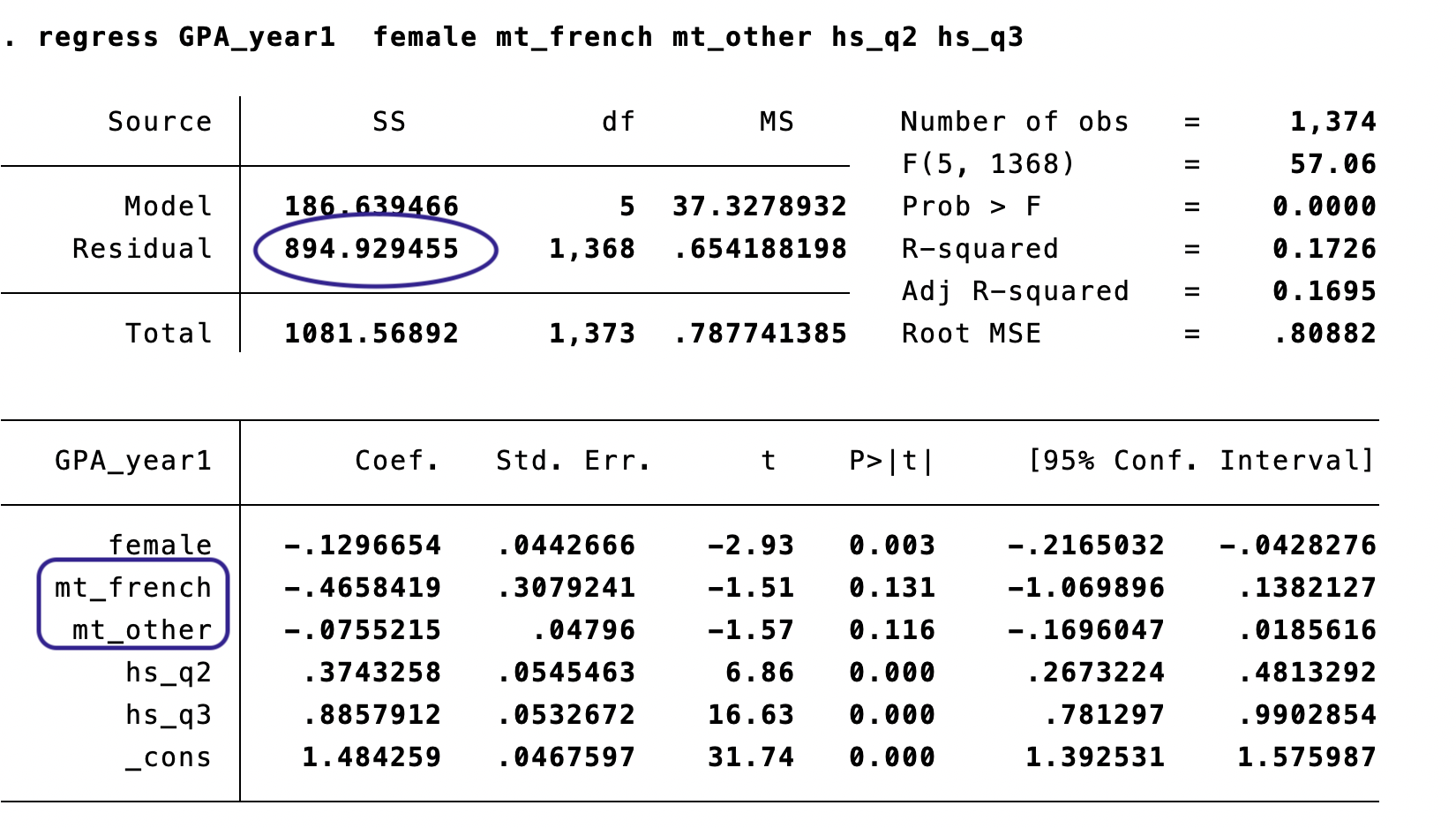
The Unrestricted Model

The full model with all variables — including the ones we’re testing:

Note the highlighted values: \(SSR_{ur} = 894.93\) and the coefficients on mt_french and mt_other.

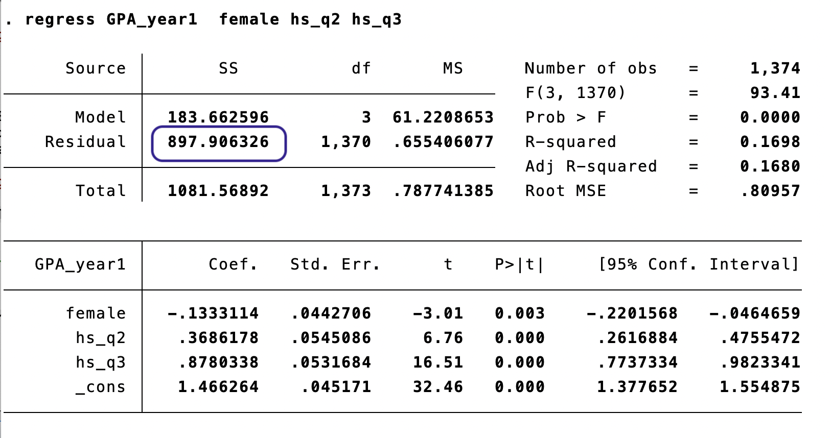
The Restricted Model

The model without mother tongue — imposing \(\beta_1 = \beta_2 = 0\):

\(SSR_r = 897.91\) — the sum of squared residuals necessarily increases when we drop variables.

But is that increase statistically significant?

The F-Statistic (Homoskedastic Version)

\[F = \frac{(SSR_r - SSR_{ur})/q}{SSR_{ur}/(n - k_{ur} - 1)} \sim F_{q, \; n-k_{ur}-1}\]

where:

  • \(q\) = number of restrictions being tested
  • \(n - k_{ur} - 1\) = degrees of freedom in the unrestricted model
  • \(SSR_r\) = sum of squared residuals from the restricted model
  • \(SSR_{ur}\) = sum of squared residuals from the unrestricted model

Intuition: The \(F\)-statistic measures the relative increase in SSR when we impose the restrictions. If the null is true, this increase should be small.

Equivalent Formula Using \(R^2\)

Since \(SSR = TSS \cdot (1 - R^2)\) and \(TSS\) is the same in both models:

\[F = \frac{(R^2_{ur} - R^2_r)/q}{(1 - R^2_{ur})/(n - k_{ur} - 1)}\]

This version is useful when regression output reports \(R^2\) but not \(SSR\).

The F-Distribution

The \(F\)-distribution:

  • Takes only positive values (reflecting that \(SSR\) can only increase when we drop variables)
  • Has two parameters: \(q\) (numerator df) and \(n - k_{ur} - 1\) (denominator df)
  • Rejection is one-sided: reject when \(F > c\)

Choose the critical value \(c\) so that the null is falsely rejected in \(\alpha\)% of cases.

Computing the F-Test: By Hand

From the Stata output: \(SSR_{ur} = 894.93\), \(SSR_r = 897.91\), \(q = 2\), \(n = 1374\), \(k_{ur} = 5\)

\[F = \frac{(897.91 - 894.93)/2}{894.93/(1374 - 5 - 1)} = \frac{2.98/2}{894.93/1368} = \frac{1.49}{0.654} = 2.28\]

\[F \sim F_{2, 1368} \quad \rightarrow \quad c_{0.10} = 2.30\]

\[P(F > 2.28) = 0.1032\]

We cannot reject the null at conventional significance levels.

The mother tongue variables are not jointly significant — we cannot conclude that mother tongue predicts GPA.

In Stata: test and testparm

After the unrestricted regression, Stata can compute the F-test directly:

* Test specific equality restrictions
test mt_french = mt_other = 0

* Or equivalently, test joint significance of a group
testparm mt_french mt_other

Both give: \(F(2, 1368) = 2.28\), \(p = 0.1032\)

Stata Tip

testparm is convenient for testing whether a group of variables is jointly significant — it sets up the \(H_0: \beta_j = 0\) for each variable in the list.

Don’t Forget Heteroskedasticity!

The F-statistic formula using \(SSR\) assumes homoskedasticity.

In practice, always estimate with robust standard errors:

regress GPA_year1 female mt_french mt_other hs_q2 hs_q3, robust
test mt_french = mt_other = 0

Robust F-test result: \(F(2, 1368) = 2.86\), \(p = 0.0573\)

Notice the Difference

Under homoskedasticity: \(F = 2.28\), \(p = 0.103\)

With robust SEs: \(F = 2.86\), \(p = 0.057\)

The robust version is closer to significance. Always use robust standard errors unless you have a specific reason not to.

Test of Overall Significance

Question: Do any of our explanatory variables predict \(y\)?

Null hypothesis: All slope coefficients are zero: \[H_0: \beta_1 = \beta_2 = \cdots = \beta_k = 0\]

Restricted model (under \(H_0\)): \[y_i = \beta_0 + u_i\] (Just the sample mean — no predictors at all)

Unrestricted model: \[y_i = \beta_0 + \beta_1 x_{1i} + \beta_2 x_{2i} + \cdots + \beta_k x_{ki} + u_i\]

The F-statistic: \[F = \frac{R^2/k}{(1 - R^2)/(n - k - 1)} \sim F_{k, \; n-k-1}\]

Why we care: If this F-test is not significant, your model explains essentially none of the variation in \(y\) — a red flag!

You’ve Been Seeing This All Along

The F(5, 1368) = 57.06 and Prob > F = 0.0000 at the top of every Stata regression output is the test of overall significance!

Usually Overwhelmingly Rejected

If your overall F-test is not significant, your model has no predictive power — a red flag!

In Stata: testparm *

You can also compute it manually after the regression:

testparm *

\[F(5, 1368) = 57.06 \qquad p = 0.0000\]

This confirms what Stata already reports at the top of the regression output.

When to Use Which Test?

t-Test vs. F-Test

Aspect t-test F-test
# of restrictions One One or more
Sided? One or two-sided Two-sided only
Use for Single coefficient Multiple coefficients

Key Relationship

When testing a single restriction: \(F = t^2\)

The results are functionally equivalent! The F-test is a generalization of the two-sided \(t\)-test to multiple restrictions.

Recipe Card: Hypothesis Tests in Multiple Regression

Type 1: One Restriction, One Coefficient

\(H_0: \beta_j = \beta_{j,0}\) (usually \(\beta_{j,0} = 0\))

  • Statistic: \(t = \frac{\hat{\beta}_j - \beta_{j,0}}{SE(\hat{\beta}_j)}\)
  • Distribution: Standard normal (large \(n\))
  • Stata: Read directly from regression output, or test varname = value

Type 2: One Restriction, Multiple Coefficients

\(H_0: \beta_j = \beta_m\)

  • Transform the regression so the restriction becomes \(\gamma_1 = 0\)
  • Or use Stata: test var1 = var2

Type 3: Joint Hypothesis (F-Test)

\(H_0: \beta_1 = 0, \; \beta_2 = 0, \; \ldots\)

  • Statistic (under homoskedasticity): \(F = \frac{(SSR_r - SSR_{ur})/q}{SSR_{ur}/(n - k_{ur} - 1)}\)
  • Distribution: \(F_{q, \; n-k_{ur}-1}\)
  • Stata: test or testparm

Key Takeaways

  1. Confidence intervals in multiple regression use the same formula as simple regression, but SEs account for other regressors

  2. Individual \(t\)-tests work for single restrictions — but don’t test one at a time when you have a joint hypothesis

  3. The F-test tests multiple restrictions simultaneously, avoiding the multiple testing problem

  4. The overall F-test is reported at the top of every regression — it tests whether all regressors are jointly significant

  5. Always use robust standard errors for heteroskedasticity-robust inference

Knowledge Check

If each of 5 individual \(t\)-tests fails to reject at the 5% level, can you conclude the variables are jointly insignificant? Why or why not?

Tip

Answer: No! The joint F-test could still reject.

Individual insignificance does not imply joint insignificance — this is precisely why we need the F-test.

Appendix: GiveDirectly Kenya Study

GiveDirectly Context: Why Cash Transfers?

The Challenge

700+ million people live on less than $2/day

Traditional Approaches - In-kind aid (food, blankets, etc.) - Conditional cash transfers (CCTs): “We give you money IF you send your kids to school / get vaccinated” - Paternalistic: Government decides what the poor “need”

Unconditional Cash Transfers (UCTs) - Direct, no strings attached - Trusts recipients to make their own decisions - Respects agency and autonomy

Why This Matters

Economic Argument

If markets work, cash is most efficient → recipients choose optimally

But markets often fail in poor areas: - Limited local supply (firms don’t invest) - Prices may spike if aggregate demand increases (inflation) - Spillovers: Money spent in one household affects neighbors

Egger, Haushofer, Miguel, Niehaus, Walker (2022)

An alternative application of hypothesis testing using field experimental data on unconditional cash transfers.

Paper: “General Equilibrium Effects of Cash Transfers: Experimental Evidence from Kenya”

Published in Econometrica 90(6):2603–2643 | 2024 Frisch Medal Winner 🏅

Research Question: What are the direct and general equilibrium effects of unconditional cash transfers?

The Study Design

Study Context

  • 653 villages in rural Kenya (Siaya County)
  • 10,500+ poor households
  • Cash transfer: ~$1,000 USD (~87,000 KES) per eligible household
  • Fiscal shock: 15% of local GDP

Randomization Strategy

  1. Village-level: Treatment vs. control villages
  2. Household-level: Eligible vs. ineligible within treatment villages
    • Eligible (thatched roof means test) → receive transfer
    • Ineligible (better housing) → NO transfer but exposed to spillovers

Main Findings

Direct Effects (on eligible recipients) - Consumption increased by 1,200-1,800 KES/month (~$12-18/month) - Assets increased substantially - Income effects from local multipliers

Spillover Effects (on ineligible neighbors) - Consumption increased by 500-1,200 KES/month (positive spillovers!) - Local firms benefited from increased demand - Minimal price inflation (no evidence of inflation eroding gains)

Local Fiscal Multiplier: 2.4 - For every dollar transferred, local economic activity increased by $2.40 - Suggests powerful local demand effects and limited import leakage

Bottom Line: Cash transfers helped both direct recipients AND their neighbors through general equilibrium effects

Regression Framework

Key Variables - treatment = 1 if household in treatment village (any status) - eligible = 1 if household eligible for transfer (means test) - ineligible = 1 if household in treatment village but ineligible - Outcome: Monthly household consumption (PPP-adjusted, KES) - Controls: Female household head, log household size, age of head (in decades)

Interaction Terms Used - treatment × eligible captures direct effect - treatment × ineligible captures spillover effect - Can test equality of these effects (Type 2 test)