Linear Regression with Multiple Regressors
SW Chapter 6
Spring 2026
Roadmap
Roadmap
- Why Multiple Regression?
- Motivation and limitations of simple regression
- The Multiple Regression Model
- Definition, OLS estimation, matrix form
- Interpreting Coefficients
- Ceteris paribus interpretation
- Examples and knowledge checks
- Omitted Variable Bias
- Derivation, formula, examples
- General cases
- Measures of Fit
- \(R^2\) and Adjusted \(R^2\)
- Model comparison
- Least Squares Assumptions
- Four assumptions for multiple regression
- Perfect multicollinearity
- Multicollinearity
- Perfect vs. imperfect
- Diagnosis and solutions
- Implementing Multiple Regression in Stata
- Syntax, detecting multicollinearity
- Partial regression plots
- Bringing It All Together
- Workflow, common pitfalls, formulas
Learning Objectives
Central Question
How do we estimate the effect of \(X_1\) on \(Y\) while holding other factors constant?
By the end of this chapter, you will:
- Estimate and interpret multiple regression models
- Understand omitted variable bias deeply
- Calculate and interpret a new measure of fit, the adjusted R²
- Recognize and handle multicollinearity
- Update our knowledge of the LS assumptions and sampling distributions of the OLS estimators when we have multiple regressors.
Why Multiple Regression?
The Limitation of Simple Regression
Recall our wage equation from Chapter 4:
\[ wage_i = \beta_0 + \beta_1 \cdot education_i + u_i \]
Problem: What’s in \(u_i\)?
- Work experience
- Ability
- Location
- Industry
- Gender, race, age…
If any of these are correlated with education, then \(\hat{\beta}_1\) suffers from omitted variable bias!
Three Reasons for Multiple Regression
- Control for confounders
- Reduce omitted variable bias
- Get closer to causal effects
- More flexible functional forms
- Include \(X^2\) and log-transformed variables for nonlinear relationships
- Interaction terms: \(X_1 \cdot X_2\)
- Better predictions
- More information \(\Rightarrow\) better forecasts
Example: Wage Equation
\[ wage_i = \beta_0 + \beta_1 \cdot education_i + \beta_2 \cdot experience_i + u_i \]
- \(\beta_1\): the effect of education on wage, holding experience constant
- \(\beta_2\): the effect of experience on wage, holding education constant
- \(u_i\): error term - what we can’t explain with education and experience
The Multiple Regression Model
Definition
Multiple Linear Regression Model
\[ Y_i = \beta_0 + \beta_1 X_{1i} + \beta_2 X_{2i} + \cdots + \beta_k X_{ki} + u_i \]
where:
- \(Y_i\): dependent variable (outcome)
- \(X_{1i}, \ldots, X_{ki}\): \(k\) independent variables (regressors)
- \(\beta_0, \ldots, \beta_k\): \(k+1\) unknown parameters
- \(u_i\): error term
OLS Estimation
Same principle as simple regression: Minimize sum of squared residuals
\[ \min_{\hat{\beta}_0, \hat{\beta}_1, \ldots, \hat{\beta}_k} \sum_{i=1}^n \hat{u}_i^2 \]
where
\[ \hat{u}_i = Y_i - \hat{\beta}_0 - \hat{\beta}_1 X_{1i} - \cdots - \hat{\beta}_k X_{ki} \]
In practice: We use statistical software (Stata, R, Python) to compute \(\hat{\beta}_0, \ldots, \hat{\beta}_k\)
Interpreting Coefficients
The Ceteris Paribus Interpretation
Partial Effect
\(\beta_j\) is the partial effect of \(X_j\) on \(Y\), holding all other regressors constant.
Mathematically:
\[ \beta_j = \frac{\partial Y}{\partial X_j} = \frac{\Delta Y}{\Delta X_j} \bigg|_{\text{other } X\text{s fixed}} \]
In words:
- “Holding \(X_2, \ldots, X_k\) constant…”
- “Controlling for \(X_2, \ldots, X_k\)…”
- “Ceteris paribus” (all else equal)
Visualizing Ceteris Paribus
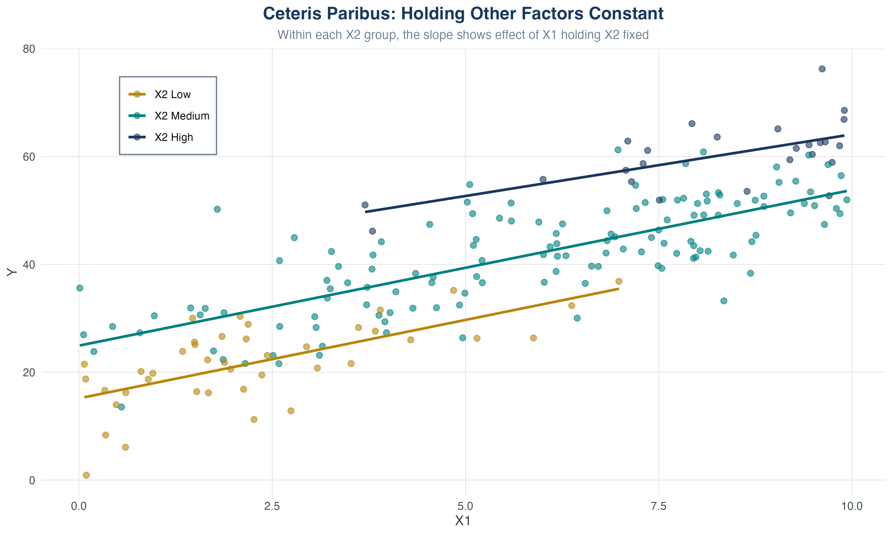
Within each \(X_2\) group, the slope shows the effect of \(X_1\) holding \(X_2\) fixed.
Example: Wage Equation
Estimated model:
wage = 5.2 + 2.1*education + 0.6*experienceInterpretation of \(\hat{\beta}_1 = 2.1\):
- Holding experience constant…
- …each additional year of education is associated with…
- …$2.10 higher hourly wage
Interpretation of \(\hat{\beta}_2 = 0.6\):
- Holding education constant…
- …each additional year of experience is associated with…
- …$0.60 higher hourly wage
Knowledge Check: Interpretation
Question
You estimate: \(colGPA = 1.3 + 0.45 \cdot hsGPA + 0.009 \cdot ACT\)
Compare two students:
- Student A: hsGPA = 3.5, ACT = 25
- Student B: hsGPA = 4.0, ACT = 25 (same ACT!)
What is the predicted difference in their college GPAs?
Answer
Difference = \(0.45 \times (4.0 - 3.5) = 0.45 \times 0.5 = 0.225\)
Student B is predicted to have a college GPA 0.225 points higher, holding ACT constant.
Example: Determinants of College GPA
Let’s look at the relationship between high school and college GPA, controlling for test scores (MSU students in Fall 1994).
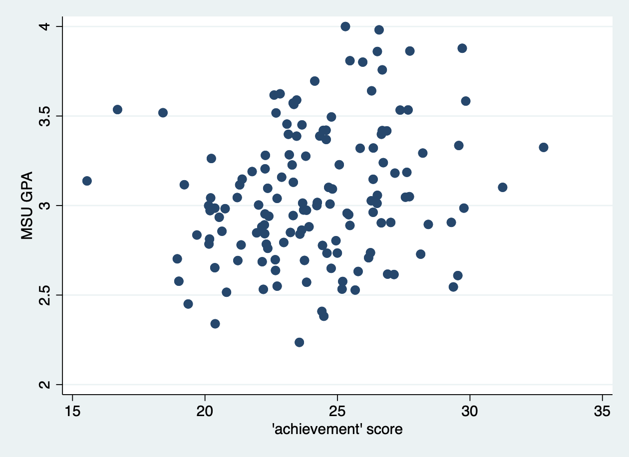
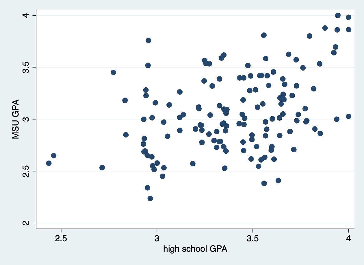
What predicts college GPA?
Example: Determinants of College GPA
We can set up the following population multiple regression model
\[ colGPA_i = \beta_0 + \beta_1 hsGPA_i + \beta_2 ACT_i + u_i \]
Example: Determinants of College GPA
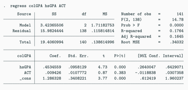
Stata regression output for college GPA
Example: Determinants of College GPA
Estimated equation (or OLS regression line):
\[ \widehat{colGPA} = 1.29 + 0.453 \cdot hsGPA + 0.0094 \cdot ACT \]
Interpretation:
- Holding ACT fixed, an additional point in high school GPA is associated with 0.453 points higher in college GPA
- Or: If we compare two students with the same ACT, but the \(hsGPA\) of student A is one point higher, we predict student A to have a \(colGPA\) that is 0.453 points higher than that of student B
Omitted Variable Bias
Omitting relevant variables: the simple case
Let’s work through some theory! True population model:
\[ Y_i = \beta_0 + \beta_1 X_{1i} + \beta_2 X_{2i} + u_i \]
Both \(X_1\) and \(X_2\) belong in the model.
But we estimate (omitting \(X_2\)):
\[ Y_i = \tilde{\beta}_0 + \tilde{\beta}_1 X_{1i} + \tilde{u}_i \]
Question
Is \(\tilde{\beta}_1\) an unbiased estimator of \(\beta_1\)?
Deriving the Bias
Assume \(X_2\) is linearly related to \(X_1\):
\[ X_{2i} = \delta_0 + \delta_1 X_{1i} + v_i \]
Substitute into the true model:
Step 1: Start with the true model:
\[ Y_i = \beta_0 + \beta_1 X_{1i} + \color{#008080}{\beta_2 X_{2i}} + u_i \]
Step 2: Replace \(X_{2i}\) with its relationship to \(X_1\):
\[ Y_i = \beta_0 + \beta_1 X_{1i} + \color{#008080}{\beta_2}(\delta_0 + \delta_1 X_{1i} + v_i) + u_i \]
Step 3: Distribute \(\color{#008080}{\beta_2}\):
\[ Y_i = \beta_0 + \beta_1 X_{1i} + \color{#008080}{\beta_2}\delta_0 + \color{#008080}{\beta_2}\delta_1 X_{1i} + \color{#008080}{\beta_2}v_i + u_i \]
Step 4: Collect like terms:
\[ \begin{aligned} Y_i &= (\beta_0 + \color{#008080}{\beta_2}\delta_0) + (\beta_1 + \color{#008080}{\beta_2}\delta_1) X_{1i} + (\color{#008080}{\beta_2}v_i + u_i) \end{aligned} \]
Omitted Variable Bias Formula
\[ E[\tilde{\beta}_1] = \beta_1 + \beta_2 \delta_1 \]
where \(\beta_2\delta_1\) is the bias.
When Does OVB Occur?
\[ \text{Bias} = \beta_2 \delta_1 \]
Bias is ZERO if:
- \(\beta_2 = 0\) (omitted variable is irrelevant)
- \(\delta_1 = 0\) (omitted variable uncorrelated with \(X_1\))
Bias is NON-ZERO when:
- Omitted variable belongs in the model (\(\beta_2 \neq 0\)), AND
- Omitted variable is correlated with included variable (\(\delta_1 \neq 0\))
Signing the Direction of Bias
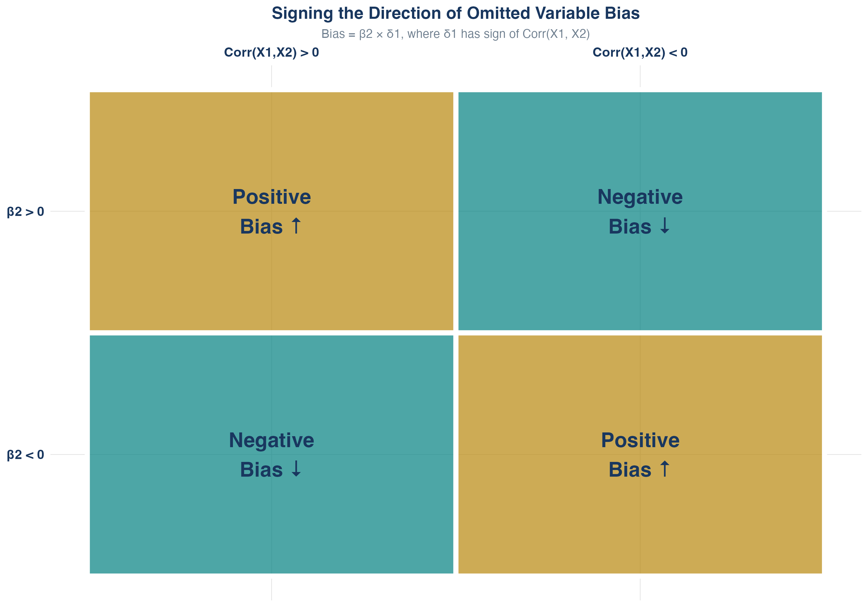
Sign of bias depends on: (1) sign of \(\beta_2\) and (2) sign of \(\text{Corr}(X_1, X_2)\). Example: Education/Ability: \(\beta_2 > 0\) and \(\text{Corr}(education, ability) > 0\) \(\Rightarrow\) positive bias
Visualizing Omitted Variable Bias
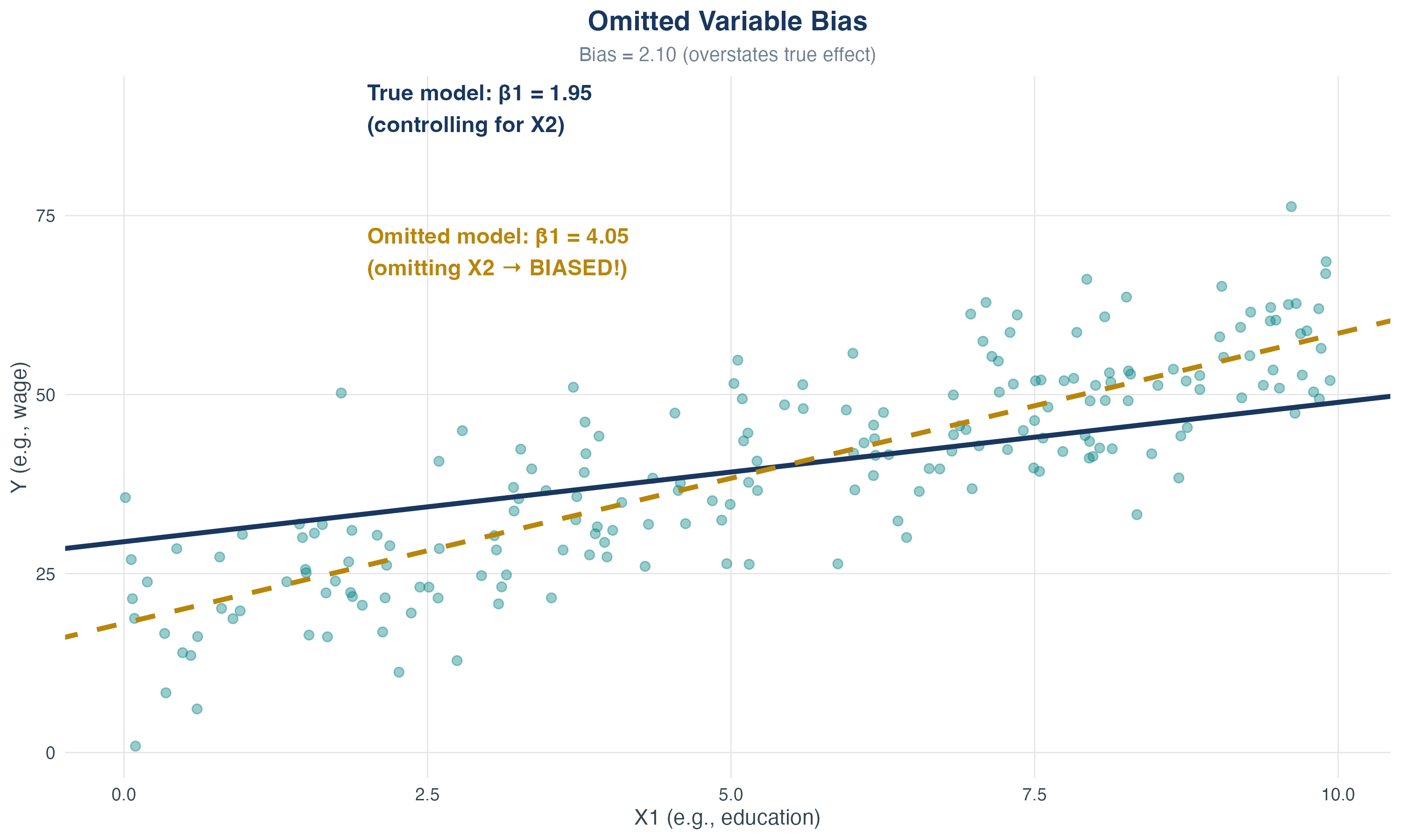
OVB: true vs omitted regression
Example: Returns to Education
True model:
\[ wage = \beta_0 + \beta_1 \cdot educ + \color{#008080}{\beta_2 \cdot abil} + u \]
But ability is unobserved!
Relationship between ability and education:
\[ \color{#008080}{abil} = \color{#008080}{\delta_0 + \delta_1 \cdot educ + v} \]
Substitute into the true model:
\[ \begin{aligned} wage &= \beta_0 + \beta_1 \cdot educ + \color{#008080}{\beta_2}(\color{#008080}{\delta_0 + \delta_1 \cdot educ + v}) + u \\ &= (\beta_0 + \color{#008080}{\beta_2\delta_0}) + (\beta_1 + \color{#008080}{\beta_2\delta_1}) \cdot educ + (\color{#008080}{\beta_2v} + u) \end{aligned} \]
What’s the bias?
- \(\beta_2 > 0\) (higher ability \(\Rightarrow\) higher wage)
- \(\delta_1 > 0\) (smarter people get more education) \(\Rightarrow\) \(\color{#008080}{\beta_2\delta_1 > 0}\)
- The return to education \(\beta_1\) will be overestimated because \(\color{#008080}{\beta_2\delta_1 > 0}\)
It will look as if people with many years of education earn very high wages, but this is partly due to the fact that people with more education are also more able on average.
Knowledge Check: OVB Direction
Question
You’re studying the effect of police officers (\(X_1\)) on crime (\(Y\)).
True model: \(crime = \beta_0 + \beta_1 \cdot police + \beta_2 \cdot poverty + u\)
You omit poverty. What’s the likely direction of bias on \(\hat{\beta}_1\)?
Hints:
- Does poverty increase crime? (sign of \(\beta_2\)?) {.fragment}
- Do high-poverty areas have more police? (sign of correlation?) {.fragment}
Answer
- \(\beta_2 > 0\) (poverty increases crime) {.fragment}
- \(\text{Corr}(police, poverty) > 0\) (more police where poverty is high) {.fragment}
- Bias = \(\beta_2 \times \delta_1 > 0\) \(\Rightarrow\) Positive bias {.fragment}
Omitting poverty makes it look like police cause crime (reverse causality illusion)! {.fragment}
OVB: More General Cases
We can extend this intuition when we add more independent variables:
\[ y = \beta_0 + \beta_1 x_1 + \beta_2 x_2 + \beta_3 x_3 + u \]
But we estimate:
\[ \widetilde{y} = \widetilde{\beta_0} + \widetilde{\beta_1} x_1 + \widetilde{\beta_2} x_2 \]
Key points:
- No general statements possible about direction of bias
- Can assume one regressor uncorrelated with others to make analysis tractable
Measures of Fit
R² in Multiple Regression
Same definition as simple regression:
\[ R^2 = \frac{ESS}{TSS} = 1 - \frac{SSR}{TSS} \]
Problem: \(R^2\) never decreases when you add regressors!
- Even if the new variable is totally irrelevant
- Even if it’s just random noise
- \(R^2\) mechanically increases (or stays constant)
This makes \(R^2\) useless for comparing models with different numbers of regressors.
Adjusted R²
Adjusted R²
\[ \bar{R}^2 = 1 - \frac{n-1}{n-k-1} \cdot \frac{SSR}{TSS} \]
where \(k\) is the number of regressors (not including intercept).
Key property: \(\bar{R}^2\) penalizes you for adding regressors
- If new variable is relevant: \(\bar{R}^2\) increases
- If new variable is irrelevant: \(\bar{R}^2\) decreases (or barely changes)
- \(\bar{R}^2 < R^2\) always
R² vs Adjusted R²
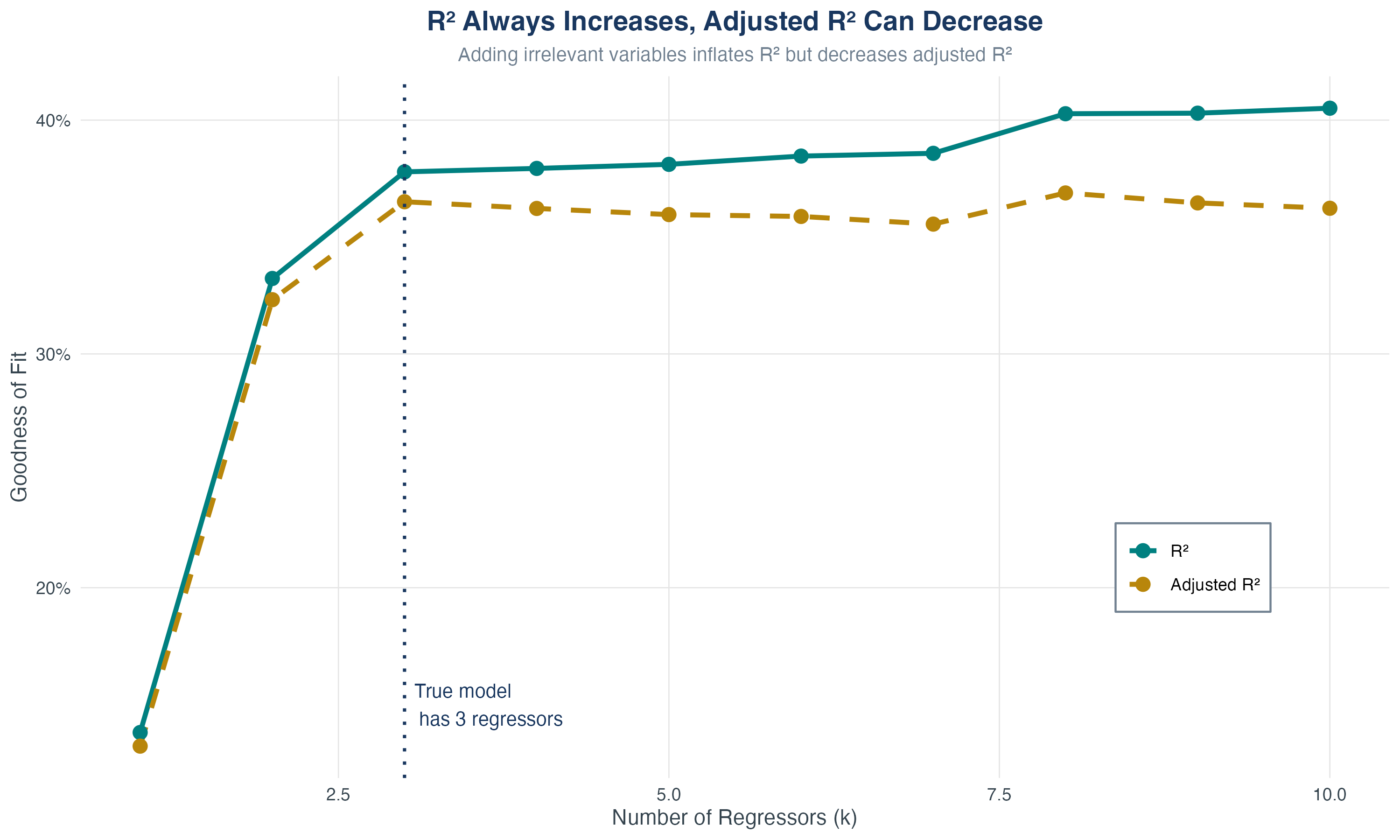
R² always increases with \(k\); adjusted R² can decrease
Knowledge Check: Calculating Adjusted R²
Question
You estimate a model with \(n = 100\) observations and \(k = 3\) regressors.
You obtain: \(SSR = 200\) and \(TSS = 500\)
Calculate the adjusted \(R^2\).
Answer
\(\bar{R}^2 = 0.5875\)
Note: \(R^2 = 0.6\), so \(\bar{R}^2 < R^2\) as expected.
Knowledge Check: Calculating Adjusted R² - Step by Step
Given: \(n = 100\), \(k = 3\), \(SSR = 200\), \(TSS = 500\)
Step 1: Write the formula:
\[ \bar{R}^2 = 1 - \frac{n-1}{n-k-1} \cdot \frac{SSR}{TSS} \]
Step 2: Plug in the values:
\[ \bar{R}^2 = 1 - \frac{100-1}{100-3-1} \cdot \frac{200}{500} \]
Step 3: Simplify:
\[ \bar{R}^2 = 1 - \frac{99}{96} \cdot \frac{200}{500} \]
Step 4: Calculate:
\[ \bar{R}^2 = 1 - 1.03125 \times 0.4 \]
\[ = 1 - 0.4125 = 0.5875 \]
Check: \(R^2 = 1 - \frac{200}{500} = 0.6\), so \(\bar{R}^2 < R^2\) as expected.
Using Adjusted R² in Practice
Model 1:
regress wage education experience
R² = 0.35, Adjusted R² = 0.34
Model 2 (adding zodiac sign):
regress wage education experience zodiac_sign
R² = 0.351, Adjusted R² = 0.339
Conclusion:
- \(R^2\) increased slightly (always does)
- Adjusted \(R^2\) decreased \(\Rightarrow\) zodiac sign is not useful!
Least Squares Assumptions
The Four LS Assumptions for Multiple Regression
We add one more assumption as we upgrade to the multiple regression model
Zero conditional mean: \(E[u_i | X_{1i}, \ldots, X_{ki}] = 0\)
i.i.d. sampling: \((X_{1i}, \ldots, X_{ki}, Y_i)\) are independently and identically distributed
Large outliers rare: \(X\)s and \(Y\) have finite fourth moments
- No perfect multicollinearity: No \(X\) is a perfect linear combination of others
Assumption 1: Zero Conditional Mean (Extended)
\[ E[u_i | X_{1i}, \ldots, X_{ki}] = 0 \]
Same interpretation as before, but now:
- Error is uncorrelated with all regressors
- Failure \(\Rightarrow\) omitted variable bias
- If an omitted variable belongs in the equation (and is in \(u\)) and it is correlated with an included \(X\), then this condition fails!
- Best solution: include the omitted variable!
Assumptions 2 and 3
Assumption 2 (\(X\)s and \(Y\) are i.i.d.):
- Satisfied automatically if the data are collected by simple random sampling
Assumption 3: Large outliers are rare:
- Same as before: \(X\)s and \(Y\) have finite fourth moments
- Check your data (scatterplots!) to make sure no crazy values
Assumption 4: No Perfect Multicollinearity (New!)
Perfect Multicollinearity
One regressor is an exact linear function of one or more other regressors.
Examples:
- \(F = \frac{9}{5}C + 32\)
- Including height in inches AND height in centimeters
- Dummy variable trap: including all categories + intercept
What happens? OLS cannot be computed (infinite solutions)
What Stata does: Automatically drops one of the collinear variables (but which one will it be?)
Perfect Multicollinearity
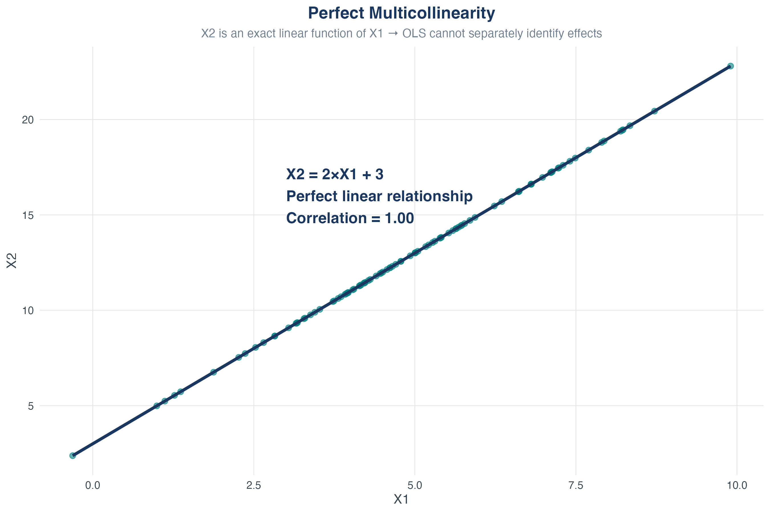
Perfect Multicollinearity
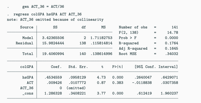
Perfect Multicollinearity
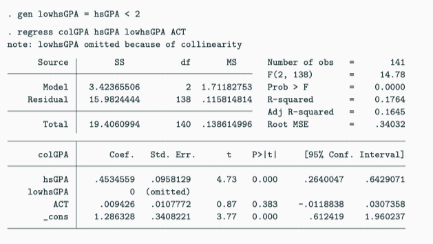
Perfect Multicollinearity - Dummy Variable Trap
Here we have a dummy variable trap:
\[ colGPA = \beta_0 + \beta_1 fresh + \beta_2 soph + \beta_3 junior \\ \qquad\quad +\ \beta_4 senior + \beta_5 hsGPA + u \]
Perfect Multicollinearity - Dummy Variable Trap
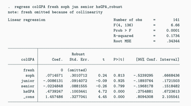
Multicollinearity
Imperfect Multicollinearity
Imperfect Multicollinearity
Two or more regressors are highly (but not perfectly) correlated.
Example: Including education AND test scores
- Correlation \(\approx 0.85\) (high, but not 1.0)
- Both can stay in the model
- But estimates will be imprecise
Why Is Imperfect Multicollinearity a Problem?
Intuition:
- \(\hat{\beta}_1\) estimates effect of \(X_1\) holding \(X_2\) constant
- But if \(X_1\) and \(X_2\) are highly correlated…
- …there’s very little variation in \(X_1\) once \(X_2\) is held constant
- Data don’t have much information about what happens when \(X_1\) changes but \(X_2\) doesn’t
Consequence: Large standard errors for \(\hat{\beta}_1\) and \(\hat{\beta}_2\)
- Coefficients not statistically significant
- This is correct — we genuinely can’t tell them apart with these data!
What to Do About Multicollinearity
Key Point
Imperfect multicollinearity is not a violation of OLS assumptions. It’s a data problem, not a method problem.
Solutions:
- Get more data (increases precision)
- Drop one of the highly correlated variables (loses information, but may be necessary)
- Combine variables (e.g., create an index)
- Accept large standard errors (honest reflection of uncertainty!)
What NOT to do: Ignore it or claim the model is “broken”
Implementing Multiple Regression in Stata
Basic Stata Syntax
Multiple regression:
Output interpretation:
- Each coefficient is a partial effect
- Standard errors are robust to heteroskedasticity
- \(R^2\) and adjusted \(R^2\) shown at bottom
Detecting Multicollinearity in Stata
Check correlations:
Bringing It All Together
The Multiple Regression Workflow
- Specify model: Which variables belong?
- Estimate: Run OLS with robust SEs
- Interpret: Partial effects (ceteris paribus)
- Assess fit: Use adjusted \(R^2\) for comparisons
- Check assumptions: Zero conditional mean, no perfect multicollinearity
- Beware OVB: Did you omit important variables?
Common Pitfalls
- Forgetting “holding other variables constant”
- Always interpret coefficients as partial effects
- Using \(R^2\) instead of adjusted \(R^2\)
- \(R^2\) is misleading when comparing models
- Ignoring omitted variable bias
- Ask: what’s in \(u\)? Is it correlated with \(X\)?
- Panicking about multicollinearity
- Large SEs are honest! They reflect genuine uncertainty
Gauss-Markov in Multiple Regression
In Chapter 5, we learned that OLS is BLUE (Best Linear Unbiased Estimator) under the Gauss-Markov conditions.
The same result extends to multiple regression — we just need one more assumption:
The Five Conditions for BLUE (Multiple Regression)
- Zero conditional mean: \(E[u_i | X_{1i}, \ldots, X_{ki}] = 0\)
- i.i.d. sampling
- Large outliers rare (finite fourth moments)
- No perfect multicollinearity
- Homoskedasticity: \(\text{Var}(u_i | X_{1i}, \ldots, X_{ki}) = \sigma^2_u\)
- Assumptions 1–4 → OLS is unbiased
- Add assumption 5 → OLS is efficient (smallest variance among linear unbiased estimators)
- If homoskedasticity fails, OLS is still unbiased — but no longer “Best”
Key Formulas Summary
| Concept | Formula |
|---|---|
| Multiple regression | \(Y = \beta_0 + \beta_1 X_1 + \cdots + \beta_k X_k + u\) |
| Partial effect | \(\beta_j = \frac{\partial Y}{\partial X_j}\) (other \(X\)s fixed) |
| OVB formula | \(E[\tilde{\beta}_1] = \beta_1 + \beta_2 \delta_1\) |
| Adjusted \(R^2\) | \(\bar{R}^2 = 1 - \frac{n-1}{n-k-1} \frac{SSR}{TSS}\) |
ECON3500 | Chapter 6