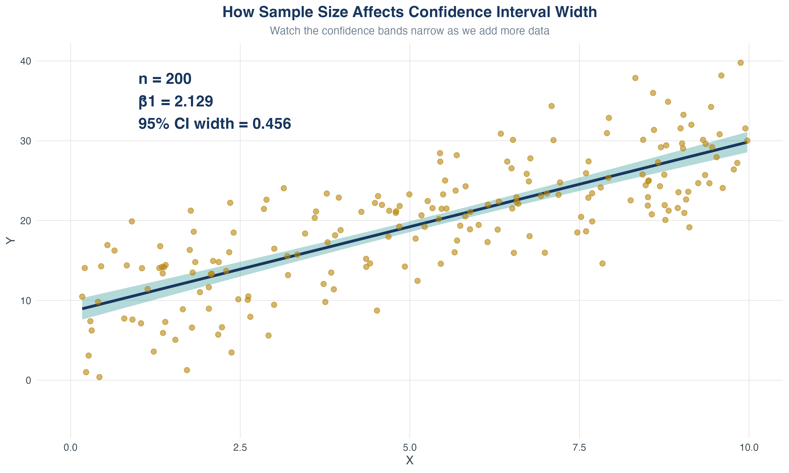
5.1 Testing Hypotheses About One Regression Coefficient
The challenge: Sampling uncertainty
Recall that \(\hat\beta_1\) is a random variable with its own sampling distribution.
- We estimated the regression coefficient (\(\hat{\beta_1}\)) of education on wages.
- But this is just one sample from the population
- If we drew a different sample, we’d get a different \(\hat{\beta_1}\)
- Question: How confident can we be that the true \(\beta_1 \neq 0\))?
Review: The Sampling Distribution of \(\hat{\beta}_1\)
Recall: under the Least Squares Assumptions, for \(n\) large, \(\hat{\beta}_1\) is approximately distributed:
\[
\hat{\beta}_1 \sim N\left(\beta_1,\;\frac{\sigma_v^2}{n(\sigma_X^2)^2}\right),\quad \text{where } v_i=(X_i-\mu_X)u_i
\]
Note: We won’t compute variances by hand, but the intuition is useful.
Key insight:
- Under 3 LS assumptions, \(\hat\beta_1\) is centered at the true \(\beta_1\) (unbiased)
- The spread (variance) depends on sample size \(n\), variation in \(X\), and error variance (\(\sigma_v^2\))
- CLT \(\Rightarrow\) \(\hat\beta_1\) is approximately normal in large samples
Hypothesis Testing: General Setup
Null hypothesis and two-sided alternative:
\[
H_0: \beta_1 = \beta_{1,0}\quad \text{vs}\quad H_1: \beta_1 \neq \beta_{1,0}
\]
Null hypothesis and one-sided alternative:
\[
H_0: \beta_1 = \beta_{1,0}\quad \text{vs}\quad H_1: \beta_1 < \beta_{1,0}
\]
where \(\beta_{1,0}\) is the hypothesized value of \(\beta_1\) under the null (usually 0).
General Approach
General formula for any hypothesis test:
\[
t = \frac{\text{estimator} - \text{hypothesized value}}{SE(\text{estimator})}
\]
- For testing \(\mu\): \(t = \frac{\bar{Y}-\mu_{Y,0}}{s_y/\sqrt{n}}\)
\[
t = \frac{\hat{\beta}_1-\beta_{1,0}}{SE(\hat{\beta}_1)}
\]
Testing \(H_0: \beta_{1,0}=0\)
Construct your \(t\)-statistic:
\[
t = \frac{\hat{\beta}_1-\beta_{1,0}}{SE(\hat{\beta}_1)}
\]
- Measures how many standard errors \(\hat\beta_1\) is away from \(\beta_{1,0}\)
- If \(|t|\) is large, \(\hat\beta_1\) is far from \(\beta_{1,0}\) \(\Rightarrow\) evidence against \(H_0\)
- Under \(H_0\), \(t \sim N(0,1)\) in large samples (rule of thumb: \(n>30\))
Decision Rule: When to Reject \(H_0\)
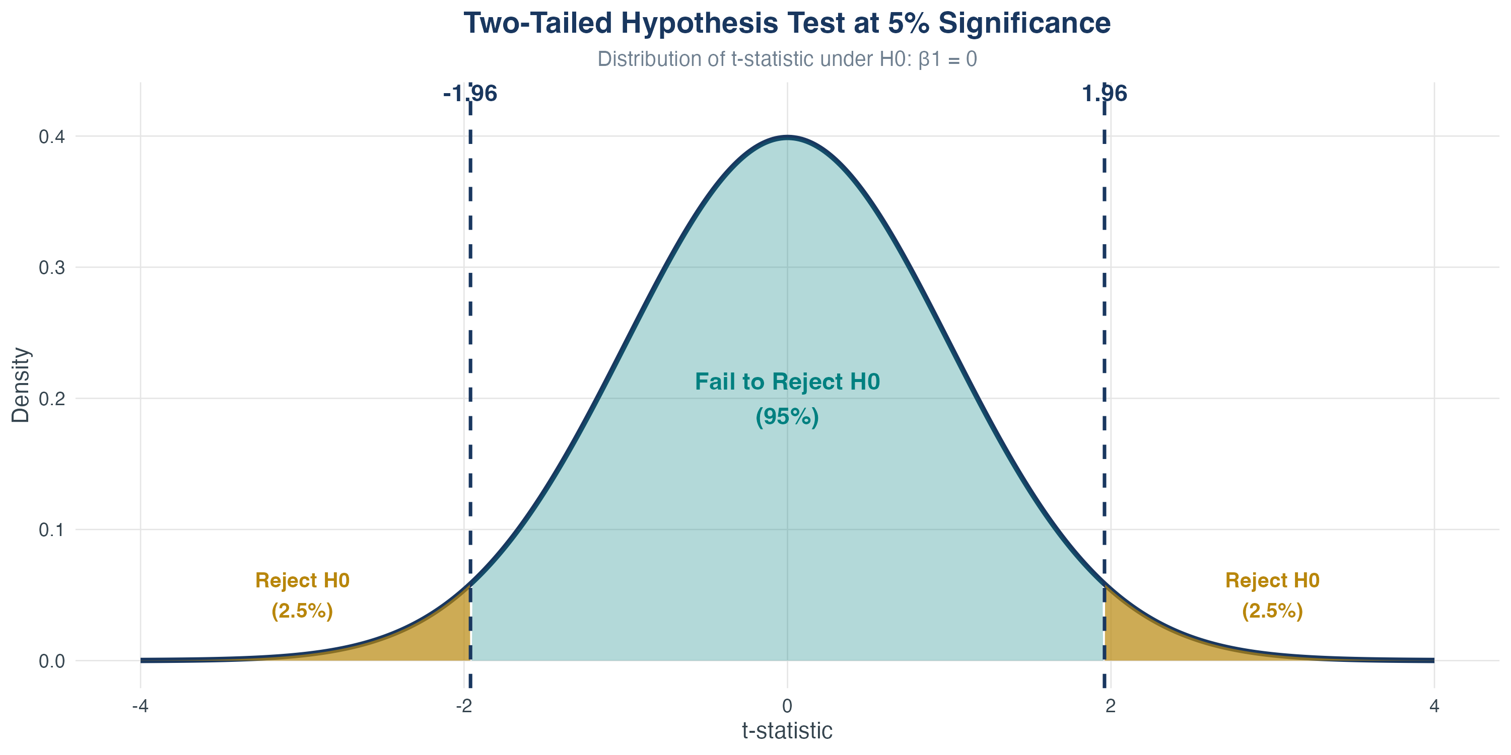
Reject \(H_0\) at significance level \(\alpha\) if:
Two-tailed: \(|t| > c_{\alpha/2}\)
One-tailed (upper): \(t > c_{\alpha}\)
One-tailed (lower): \(t < -c_{\alpha}\)
In practice, almost always two-tailed tests
Common critical values:
| 1% |
0.01 |
2.58 |
| 5% |
0.05 |
1.96 |
| 10% |
0.10 |
1.645 |
Choosing a Significance Level
- We fix \(\alpha\) as the significance level (Type I error)
- \(\alpha\) is the probability of falsely rejecting the null
- Typical choice: \(\alpha=0.05\) (5% false positives)
- Is that too high? Why not make \(\alpha\) super small?
Choosing a Significance Level (Tradeoff)
- Smaller \(\alpha\) makes it harder to reject \(H_0\)
- Fewer false positives, but more false negatives
- Power = \(1-\beta\) (probability of rejecting a false null)
- Tradeoff between significance (\(\alpha\)) and power (\(\beta\))
Decision Rule: When to Reject \(H_0\)
Rejection regions for one- and two-sided tests
Reject \(H_0\) at significance level \(\alpha\) if:
- Two-tailed: \(|t| > c_{\alpha/2}\)
- One-tailed (upper): \(t > c_{\alpha}\)
- One-tailed (lower): \(t < -c_{\alpha}\)
One-Tailed vs Two-Tailed Tests
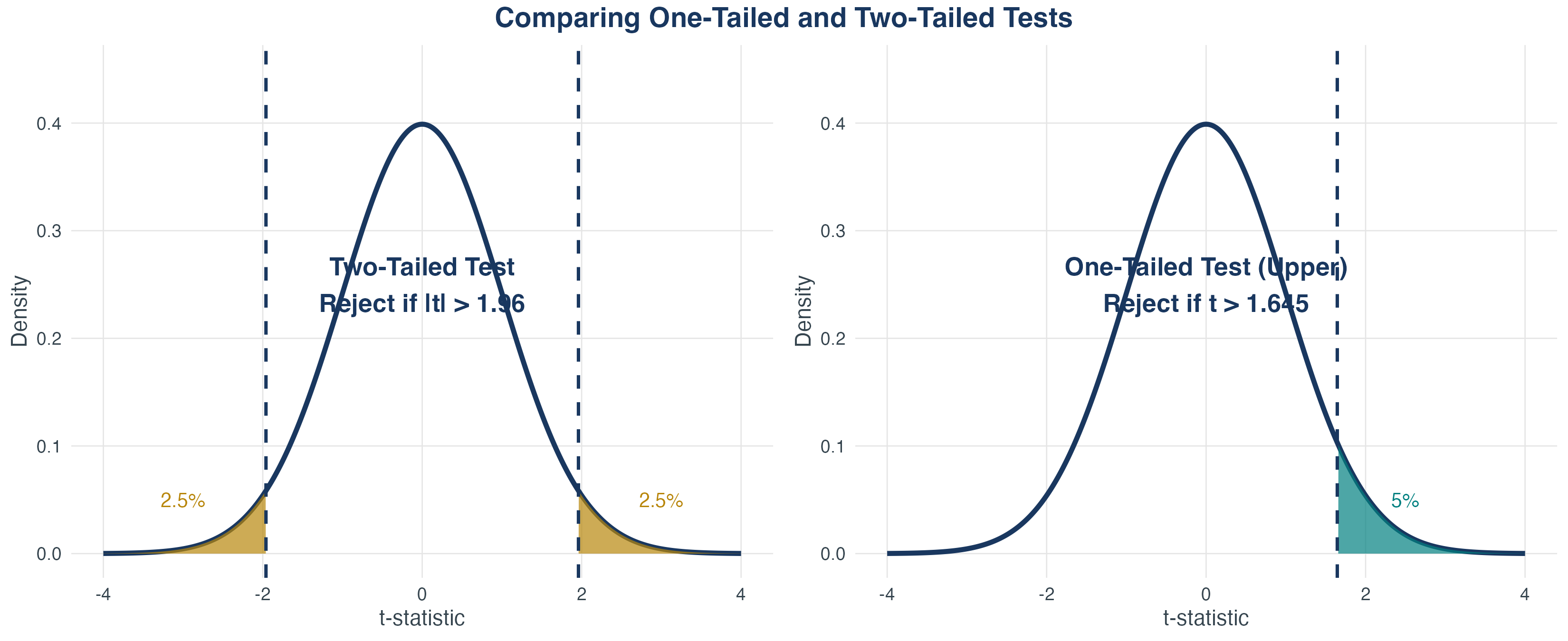
Which to use?
- Two-tailed: Most common in economics (test for any effect)
- One-tailed: When theory strongly predicts a direction
Critical Values for Common Significance Levels
| 10% |
1.645 |
1.28 |
| 5% |
1.96 |
1.645 |
| 1% |
2.58 |
2.33 |
Rule of thumb: For two-tailed tests at 5%, reject if \(|t| > 2\).
Type I and Type II Errors
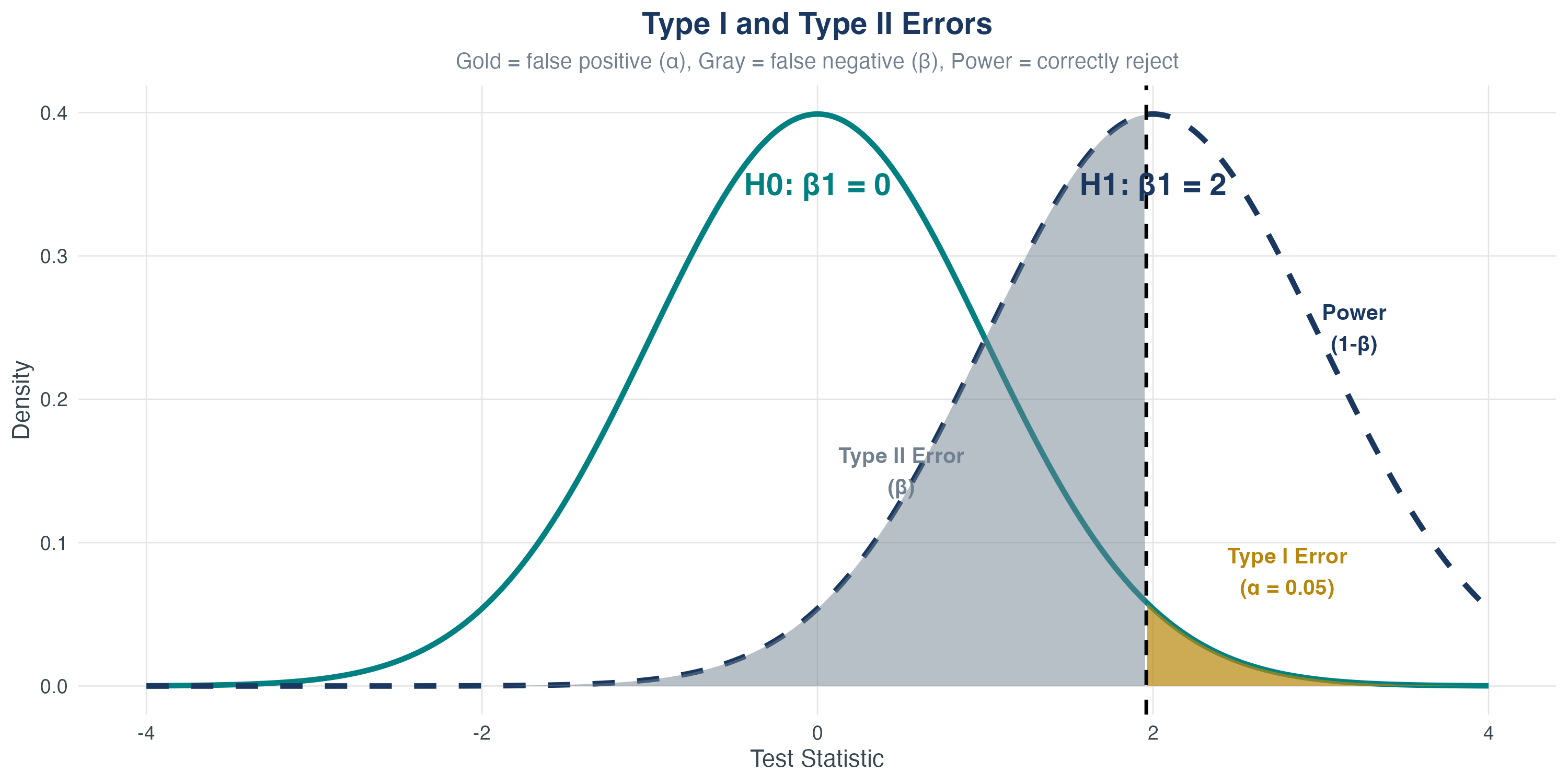
Type I and Type II errors
- Type I error (\(\alpha\)): Reject \(H_0\) when it’s true (false positive)
- Type II error (\(\beta\)): Fail to reject \(H_0\) when it’s false (false negative)
- Power \((1-\beta)\): Probability of correctly rejecting false \(H_0\)
Choosing a Significance Level
Why \(\alpha = 0.05\) is conventional
- We tolerate a 5% chance of false positives
- Balances Type I and Type II errors
- Widely accepted standard in social sciences
The tradeoff
- Smaller \(\alpha\) \(\Rightarrow\) fewer false positives, but more false negatives (lower power)
- Larger \(\alpha\) \(\Rightarrow\) more false positives, but fewer false negatives (higher power)
- You cannot minimize both at once.
We typically fix \(\alpha\) and try to increase power by increasing \(n\).
Statistical Power
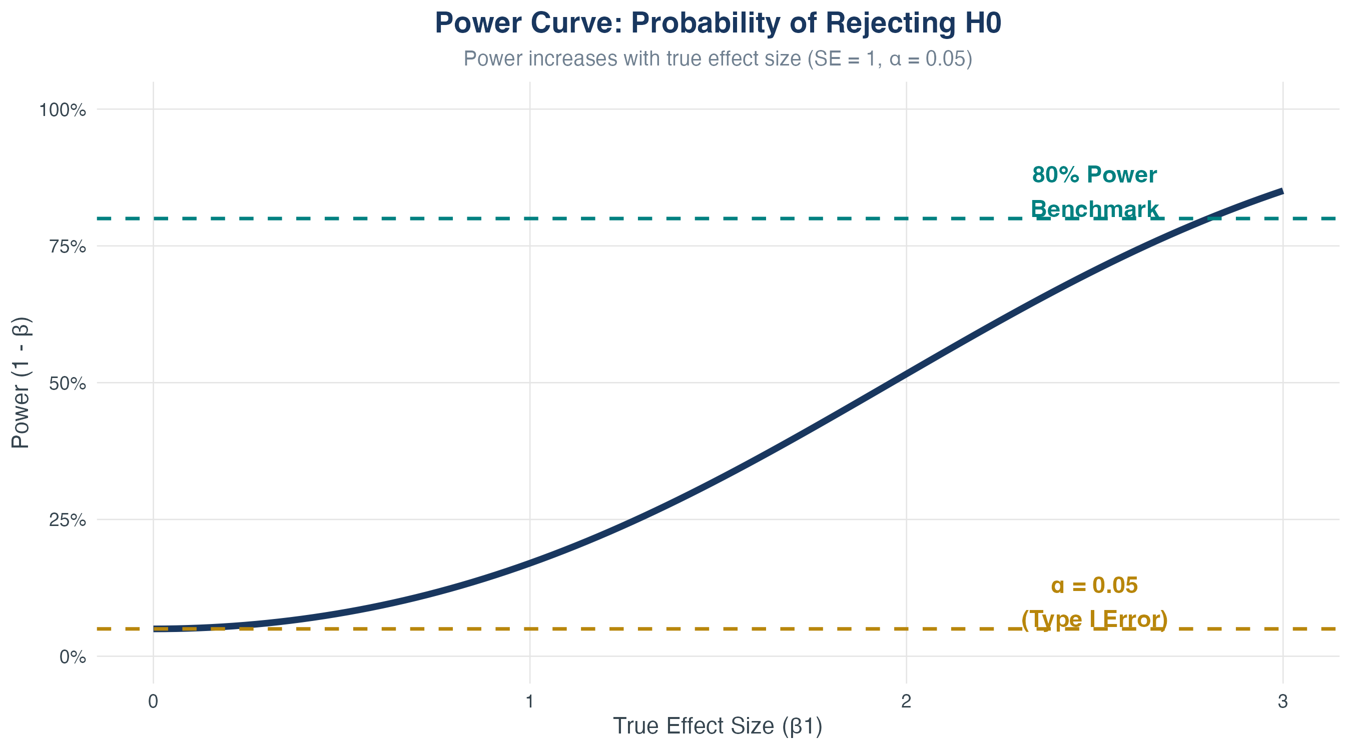
Power increases with:
- Larger true effect size \(|\beta_1|\)
- Larger sample size \(n\)
- Smaller error variance \(\sigma^2_u\)
Understanding \(p\)-Values
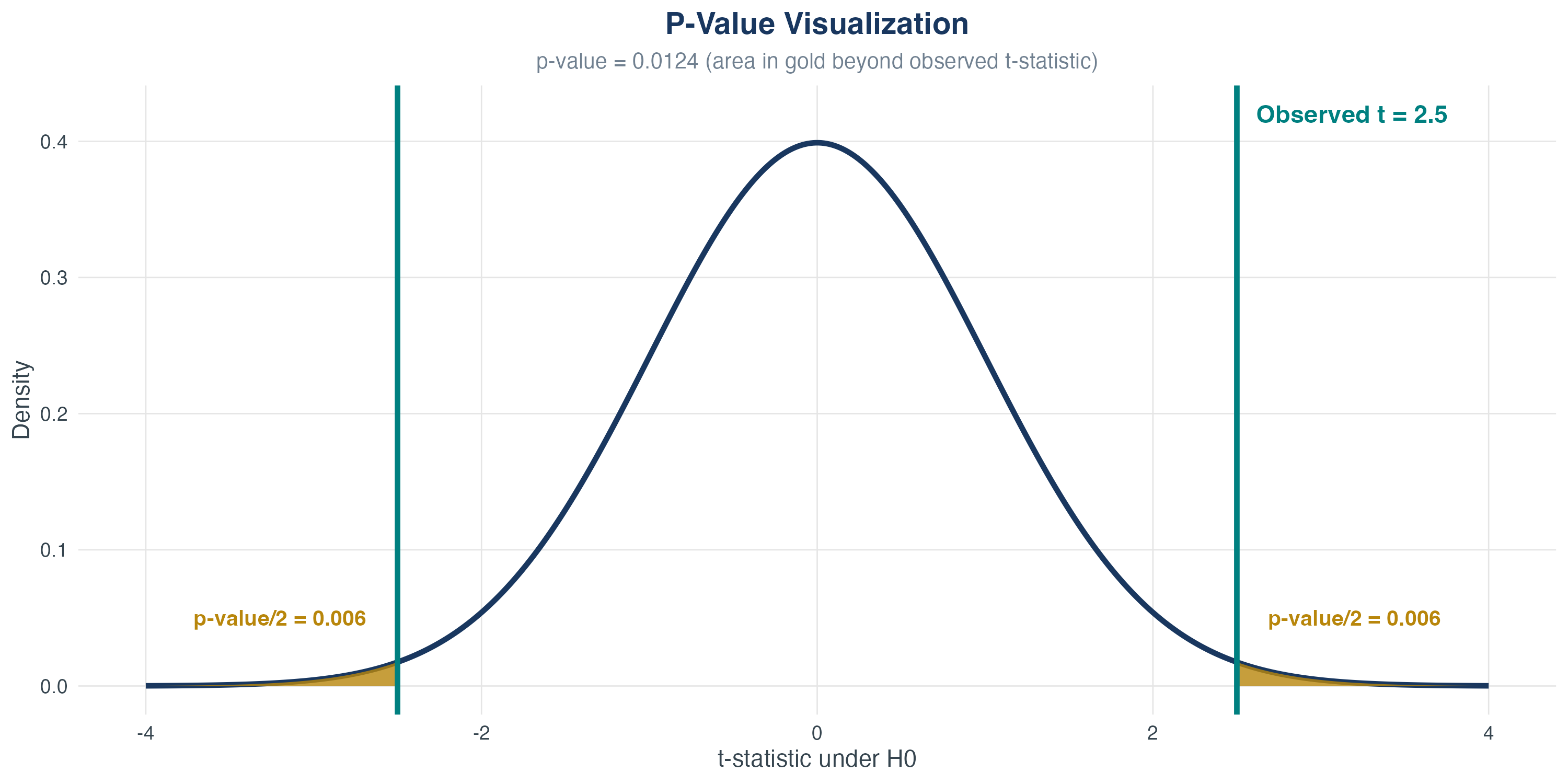
\(p\)-value interpretation
- Probability of observing a \(t\)-statistic this extreme (or more) if \(H_0\) is true
- Smaller \(p\)-value \(\Rightarrow\) stronger evidence against \(H_0\)
- Reject \(H_0\) if \(p\text{-value} < \alpha\)
Hypothesis Testing in Stata
Testing \(H_0: \beta_1 = 0\)
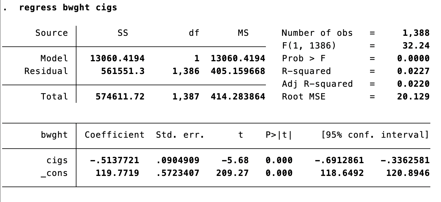
Stata output automatically shows:
- Coefficient estimate \(\hat\beta_1\)
- Standard error \(\operatorname{SE}(\hat\beta_1)\)
- \(t\)-statistic \(t = \hat\beta_1 / \operatorname{SE}(\hat\beta_1)\)
- \(p\)-value: probability of observing \(|t|\) this large if \(H_0\) is true
Decision rule using \(p\)-value
- Reject \(H_0\) if \(p\)-value < \(\alpha\)
- Equivalent to checking if \(|t| > c_{\alpha/2}\)
Testing \(H_0: \beta_1 = a\) (Non-Zero Null)
What if we want to test a different null value?
Suppose we hypothesize that an extra year of education increases wage by exactly $3/hour:
\[
H_0: \beta_1 = 3 \quad \text{vs} \quad H_1: \beta_1 \neq 3.
\]
Modified \(t\)-statistic:
\[
t = \frac{\hat\beta_1 - 3}{\operatorname{SE}(\hat\beta_1)}.
\]
Example
- If \(\hat\beta_1 = 2.5\) and \(\operatorname{SE}(\hat\beta_1) = 0.4\), then \(t = (2.5 - 3)/0.4 = -1.25\)
- Since \(|-1.25| < 1.96\), fail to reject \(H_0: \beta_1 = 3\)
- Not enough evidence to say the effect differs from $3
Economic vs Statistical Significance
Statistical significance \(\neq\) economic significance.
Scenario 1: Statistically significant but economically trivial
- \(\hat\beta_1 = 0.05\), \(\operatorname{SE}(\hat\beta_1) = 0.01\), \(t = 5\) (highly significant!)
- An extra year of education increases wage by 5 cents/hour
- Technically significant, but economically negligible
Scenario 2: Economically important but statistically insignificant
- \(\hat\beta_1 = 8\), \(\operatorname{SE}(\hat\beta_1) = 10\), \(t = 0.8\) (not significant)
- Small sample \(\Rightarrow\) high uncertainty
- Effect could be large, but we can’t be confident
Takeaway: Always examine both statistical significance and magnitude.
Conducting a Hypothesis Test
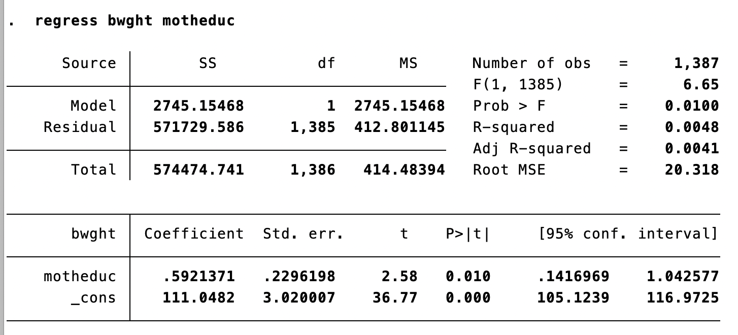
Is mother’s education associated with birthweight?
Testing \(H_0: \beta_1 = a\)
\[H_0: \beta_1 = a\] \[H_1: \beta_1 \neq a\]
Adjust the \(t\)-statistic
\[
t = \frac{\hat{\beta}_1 - a}{SE(\hat{\beta}_1)}
\]
5.3 Regression When \(X\) Is Binary
Regression When \(X\) Is Binary
Often, our regressor takes only two values:
- \(X = 1\) if small class, \(X = 0\) if large class
- \(X = 1\) if treated, \(X = 0\) if control
- \(X = 1\) if college degree, \(X = 0\) if no degree
- \(X = 1\) if female, \(X = 0\) if male
These are called binary variables, dummy variables, or indicator variables.
Terminology
- \(X = 1\): “treatment group” or “category of interest”
- \(X = 0\): “control group” or “reference category”
Gender is not binary, but it is recorded as binary in many datasets—data availability shapes our understanding of the world.
Interpreting a Binary \(X\)
Population model: \(Y_i = \beta_0 + \beta_1 X_i + u_i\)
When \(X_i=0\):
\(Y_i = \beta_0 + \beta_1 * 0+ u_i\)
\(E[Y_i\mid X_i=0]=E[\beta_0 + u_i]=E[\beta_0] + E[u_i]= \beta_0\)
\(Y_i = \beta_0 + \beta_1 + u_i\)
\(Y_i = \beta_0 + \beta_1 * 1+ u_i\)
\(Y_i = \beta_0 + \beta_1 + u_i\)
\(E[Y_i\mid X_i=1]=E[\beta_0 + \beta_1 + u_i]=E[\beta_0] + E[\beta_1] + E[u_i]= \beta_0 + \beta_1\)
Interpreting a Binary \(X\)
Therefore:
\[
\beta_1 = E(Y_i\mid X_i=1) - E(Y_i\mid X_i=0)
\]
So \(\beta_1\) is the population difference in group means.
Interpreting a Binary \(X\): Stata Output
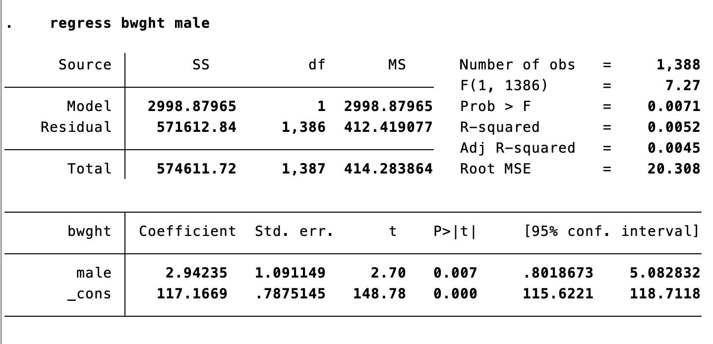
Is sex associated with birthweight?
Interpreting a Binary \(X\) (Example)
Is sex associated with birthweight?
\[\hat{bwght} = 117.17 + 2.94\,male\]
- Average birthweight of female babies: \(E[bwght\mid male=0] = 117.17\) ounces
- Average birthweight of male babies: \(E[bwght\mid male=1] = 117.17 + 2.94 = 120.11\) ounces
5.4 Heteroskedasticity and Homoskedasticity
Homoskedasticity in a Picture
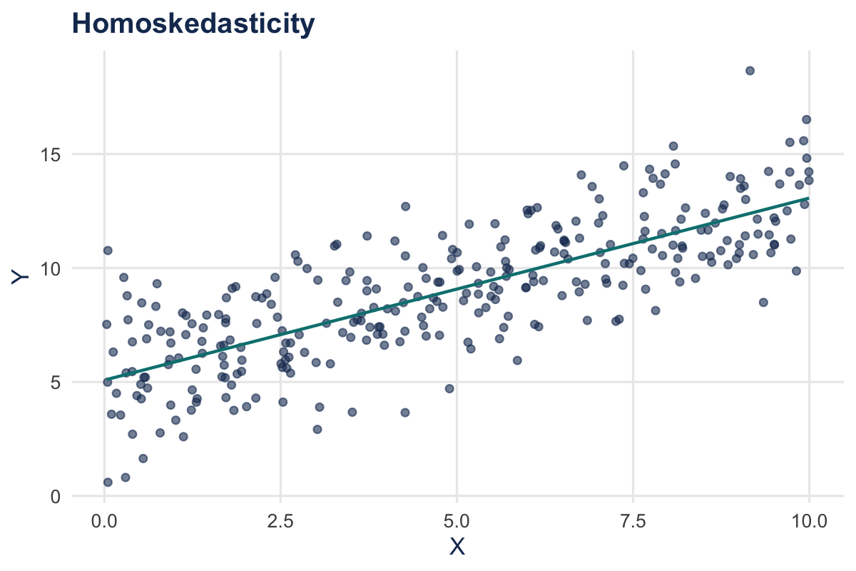
- The variance of \(u\) is constant
- The variance of \(u\) does not depend on \(X\)
Heteroskedasticity in a Picture
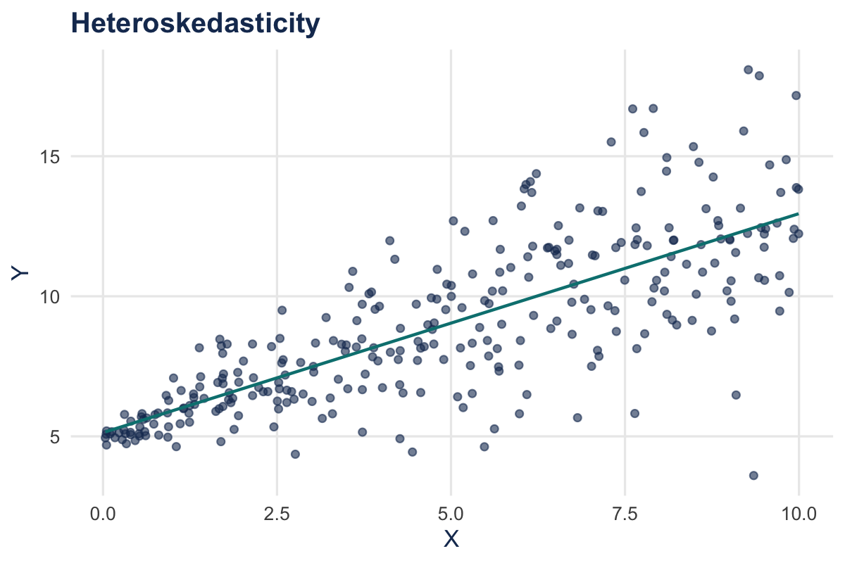
- The variance of \(u\) is not constant
- The variance of \(u\) does depend on \(X\)
So Who Cares?
Heteroskedasticity does not affect point estimates of \(\beta_1\).
But it does affect your standard errors.
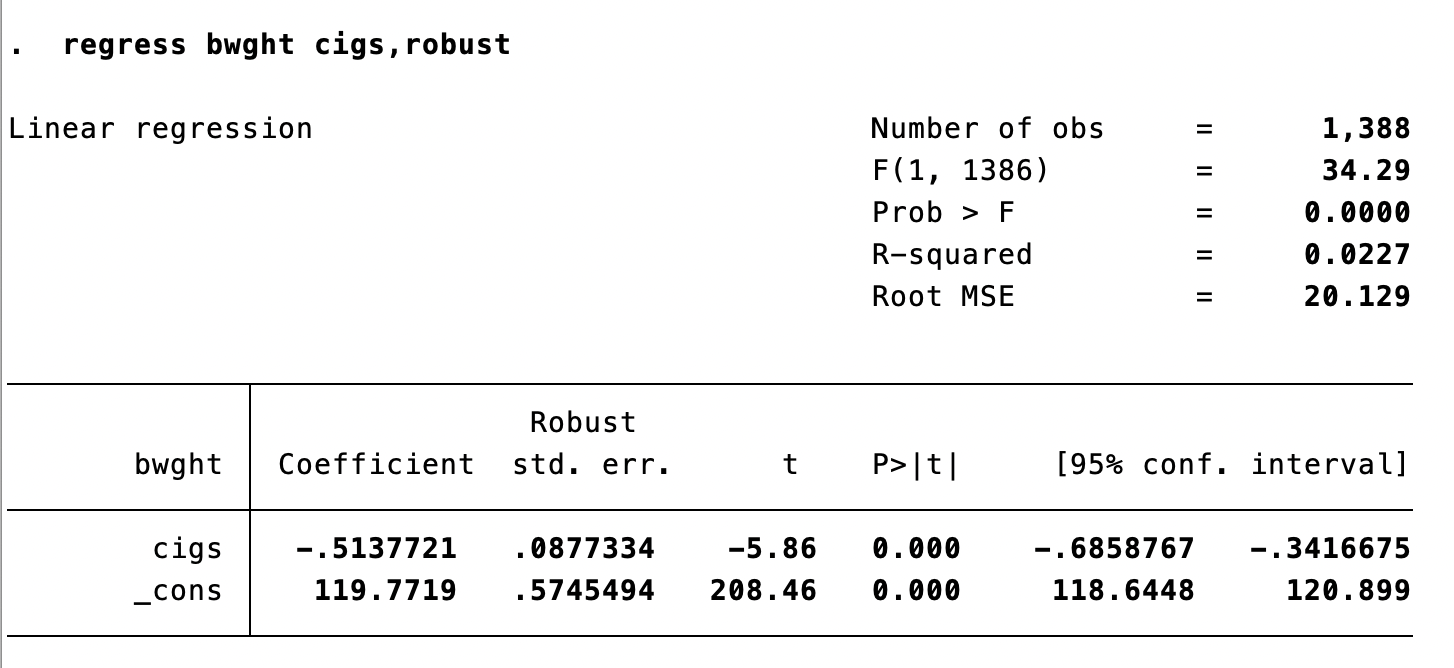
Homoskedastic-only standard errors are unbiased only under homoskedasticity. We adjust using heteroskedasticity-robust standard errors.
Heteroskedasticity-Robust Standard Errors (Stata)
Heteroskedasticity-Robust Standard Errors (Stata)
Comparing Homoskedastic and Robust SEs
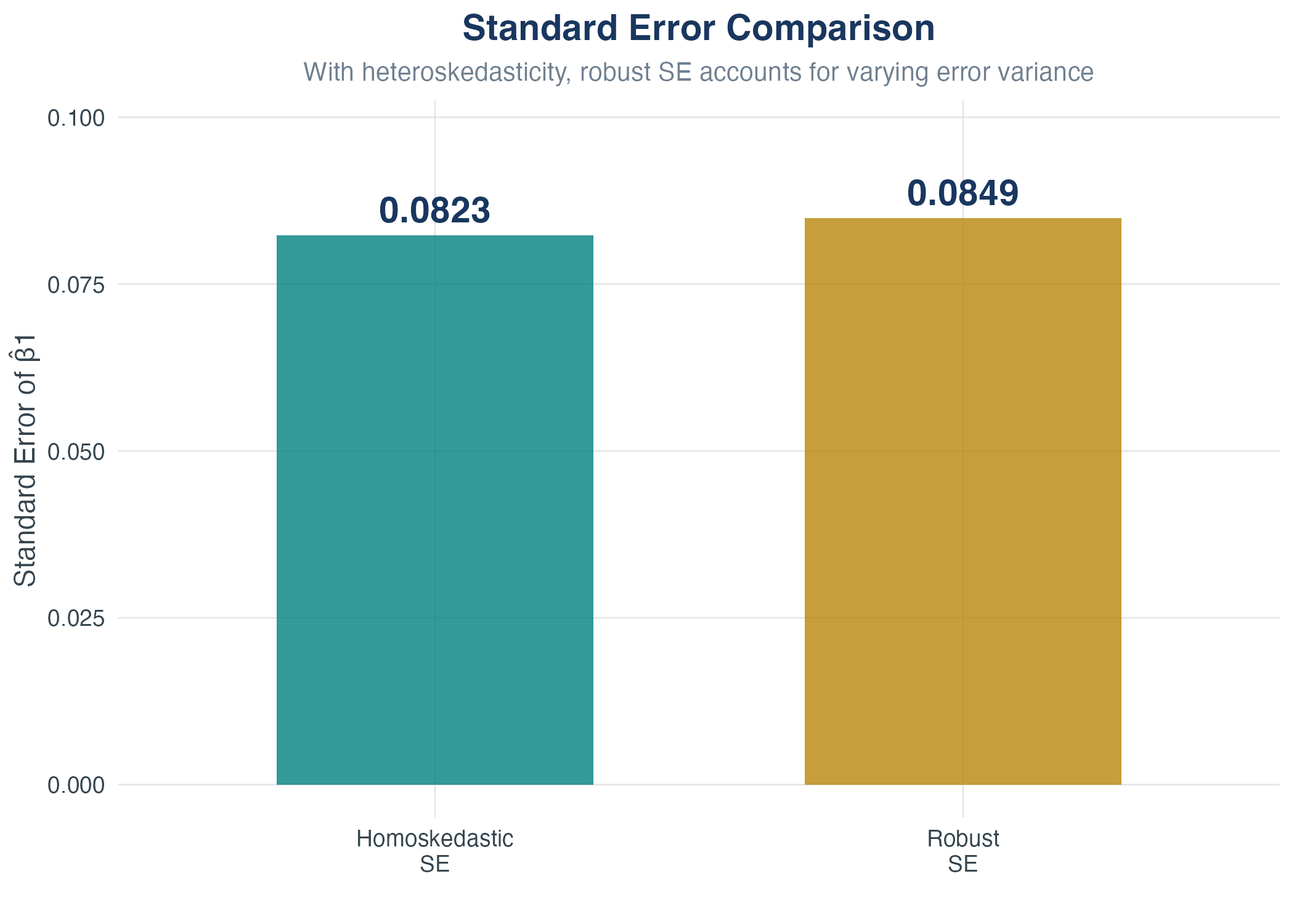
- In this example with heteroskedasticity, robust SE is larger
- But this isn’t always the case – it can go either way
- Always use robust SEs as a precaution
Heteroskedasticity: The Bottom Line
| Errors are homoskedastic |
Correct |
Correct |
| Errors are heteroskedastic |
Wrong |
Correct |
Always use robust standard errors.
No downside if errors are homoskedastic, protects you if they’re not.