Linear Regression with One Regressor

Chapter 4

ECON3500: Econometrics and Applications

Spring 2026

Learning Roadmap

The Central Question

How do we move from observing relationships in data to making predictions and testing causal claims?

By the end of this chapter, you will be able to:

• Set up and estimate a simple linear regression model
• Interpret slopes and intercepts with precision
• Calculate and understand fitted values and residuals
• Assess model quality using R², TSS, ESS, SSR, and SER
• State the key assumptions behind OLS estimation
• Implement everything in Stata

Our Journey

1. The linear regression model
2. Estimating coefficients: ordinary least squares
3. Measuring how well the model fits
4. Assumptions for unbiased estimates
5. Sampling distributions and uncertainty
6. Common misconceptions and clarifications
7. Implementing OLS in Stata
8. Bringing it all together

The Linear Regression Model

Motivating Question

Returns to education

What are the economic returns to education?

Why this matters:

• We observe that more educated people tend to earn more

• Is this just correlation, or something more?

• How much more do we expect someone with 16 years of education to earn vs. someone with 12 years?

• Can we quantify the relationship systematically?

Our goal: Move from vague observations to a prediction rule we can compute from data.

Data Source

Example data: Education and Annual Wages

Source: American Community Survey (ACS) 2024 Sample: 300 observations

Variables: Education: Years of schooling (8-20 years) Wages: Annual earnings in thousands of 2024 dollars

Note: Based on realistic patterns from ACS microdata

First Look at the Data

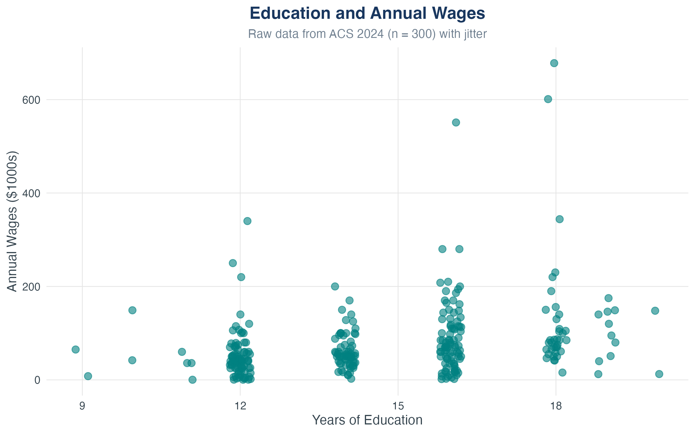
What do you see?

• Each point is one person’s (education, wages) pair
• General upward trend (positive relationship)
• Lots of scatter (other factors matter too!)

From Picture to Model

Three tools for describing relationships:

1. Scatter plots give us a first look

2. Correlation tells us direction and strength

3. Linear regression gives us a mathematical summary we can use for prediction

Key Insight

Regression transforms a cloud of points into an equation. That equation becomes a model we can interrogate, test, and use.

What Regression Analysis Does

Regression helps us:

• Predict: Given someone’s education, what wages would we expect?

• Explain: How does a one-year change in education map to wage changes?

• Control: What’s the education-wages relationship holding other factors fixed?

Vocabulary:

• Dependent variable (\(Y\)): the outcome we want to explain (wages)
• Independent variable (\(X\)): the driver we use to explain it (education)

The Population Model

In the population, the true relationship is: \[ Y = \beta_0 + \beta_1 X + u \]

Components:

• \(\beta_0\): intercept — baseline level of \(Y\) when \(X = 0\)

• \(\beta_1\): slope — change in \(Y\) from a one-unit increase in \(X\)

• \(u\): error term — all other influences on \(Y\) not captured by \(X\)

\(\blacktriangleright\) This is a model — a simplified representation of reality. Our job: estimate \(\beta_0\) and \(\beta_1\) from data.

Understanding the Error Term

\[ \text{Wages} = \beta_0 + \beta_1 \cdot \text{Education} + u \]

What’s in \(u\)?

• Ability and talent
• Work experience
• Gender
• Family background
• Pure luck
• Measurement error

Critical Point

We can’t observe \(u\), but its properties determine whether we can interpret \(\beta_1\) causally. More on this later.

Ceteris Paribus: Holding Other Things Fixed

Ceteris paribus = “other things equal”

\[ Y = \beta_0 + \beta_1 X + u \]

Taking changes: \[ \Delta Y = \beta_1 \Delta X + \Delta u \]

Holding \(u\) fixed means \(\Delta u = 0\): \[ \Delta Y = \beta_1 \Delta X \]

Slope Interpretation

\(\beta_1\) is the change in \(Y\) associated with a one-unit change in \(X\), holding all other factors (captured in \(u\)) fixed.

The Regression Line in Action

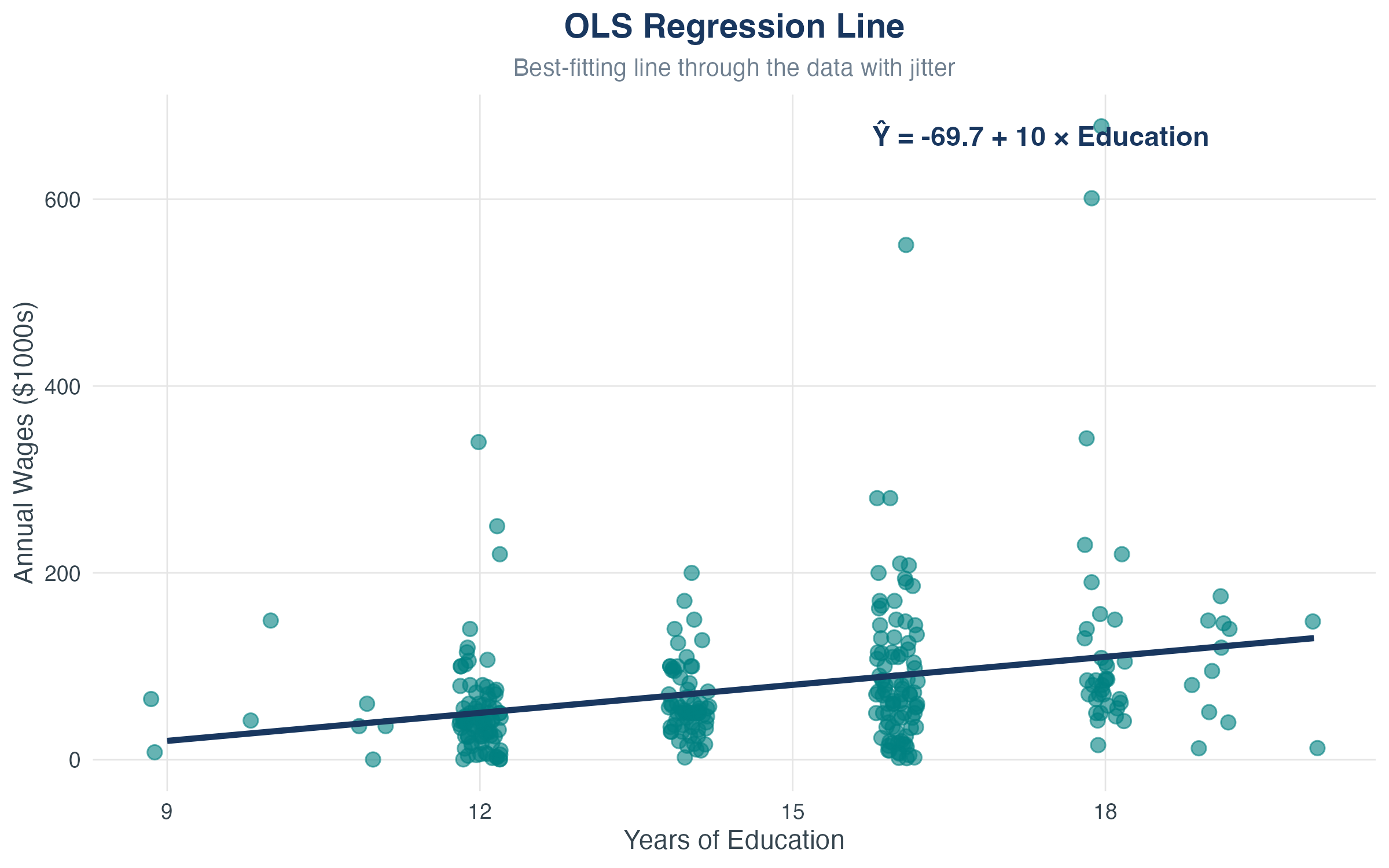
The line is: \(\hat{Y} = \hat{\beta}_0 + \hat{\beta}_1 X\)

• Best linear summary of the scatter
• Every vertical deviation from the line is a residual

Estimating Coefficients: Ordinary Least Squares

From Population to Sample

The challenge:

• In the population: \(Y_i = \beta_0 + \beta_1 X_i + u_i\)

• We observe \((X_i, Y_i)\) for \(i = 1, \ldots, n\)

• We do not observe \(u_i\)

• We must estimate \(\beta_0\) and \(\beta_1\) from the sample

Notation:

• \(\hat{\beta}_0\), \(\hat{\beta}_1\) = our estimates (the “hats” indicate estimates)
• Goal: Make these estimates as close as possible to the true \(\beta_0\), \(\beta_1\)

The OLS Criterion

Idea: Choose \(\hat{\beta}_0\) and \(\hat{\beta}_1\) to make prediction errors as small as possible.

For each observation, the prediction error is: \[ Y_i - (\beta_0 + \beta_1 X_i) \]

OLS minimizes the sum of squared errors: \[ \min_{\beta_0, \beta_1} \sum_{i=1}^{n} \left[ Y_i - (\beta_0 + \beta_1 X_i) \right]^2 \]

Why square?

• Positive and negative errors don’t cancel out
• Penalizes large mistakes more than small ones
• Leads to a closed-form solution (calculus magic!)

Deriving the OLS Estimators [Optional]

For Math Lovers

This derivation uses calculus to show where the OLS formulas come from. Feel free to skip if you prefer!

Setup: Minimize the sum of squared residuals \[ S(\beta_0, \beta_1) = \sum_{i=1}^{n} \left[ Y_i - (\beta_0 + \beta_1 X_i) \right]^2 \]

Step 1: Take first-order conditions (FOCs) \[ \begin{aligned} \frac{\partial S}{\partial \beta_0} &= -2 \sum_{i=1}^{n} \left[ Y_i - (\beta_0 + \beta_1 X_i) \right] = 0 \\[0.3em] \frac{\partial S}{\partial \beta_1} &= -2 \sum_{i=1}^{n} X_i \left[ Y_i - (\beta_0 + \beta_1 X_i) \right] = 0 \end{aligned} \]

Step 2: Solve the first equation for \(\hat{\beta}_0\) \[ \begin{aligned} \sum Y_i &= n\hat{\beta}_0 + \hat{\beta}_1 \sum X_i \\ \hat{\beta}_0 &= \frac{1}{n}\sum Y_i - \hat{\beta}_1 \frac{1}{n}\sum X_i = \bar{Y} - \hat{\beta}_1 \bar{X} \end{aligned} \]

Deriving the OLS Estimators (continued)

Step 3: Substitute \(\hat{\beta}_0\) into the second FOC \[ \begin{aligned} \sum X_i Y_i &= \hat{\beta}_0 \sum X_i + \hat{\beta}_1 \sum X_i^2 \\ \sum X_i Y_i &= (\bar{Y} - \hat{\beta}_1 \bar{X}) \sum X_i + \hat{\beta}_1 \sum X_i^2 \\ \sum X_i Y_i &= \bar{Y} n\bar{X} - \hat{\beta}_1 n\bar{X}^2 + \hat{\beta}_1 \sum X_i^2 \end{aligned} \]

Step 4: Solve for \(\hat{\beta}_1\) \[ \begin{aligned} \hat{\beta}_1 \left( \sum X_i^2 - n\bar{X}^2 \right) &= \sum X_i Y_i - n\bar{X}\bar{Y} \\[0.3em] \hat{\beta}_1 &= \frac{\sum X_i Y_i - n\bar{X}\bar{Y}}{\sum X_i^2 - n\bar{X}^2} = \frac{\sum(X_i - \bar{X})(Y_i - \bar{Y})}{\sum(X_i - \bar{X})^2} \end{aligned} \]

Result: This is the formula for \(\hat{\beta}_1\) in “The OLS Formulas” slide!

The OLS Formulas

Solution from calculus (see previous slides for derivation):

\[ \begin{aligned} \hat{\beta}_1 &= \frac{\sum_{i=1}^{n}(X_i - \bar{X})(Y_i - \bar{Y})}{\sum_{i=1}^{n}(X_i - \bar{X})^2} = \frac{\text{Cov}(X,Y)}{\text{Var}(X)} \\[0.5em] \hat{\beta}_0 &= \bar{Y} - \hat{\beta}_1 \bar{X} \end{aligned} \]

Intuition:

• \(\hat{\beta}_1\) depends on how \(X\) and \(Y\) covary

• Need variation in \(X\) to estimate \(\beta_1\) (if all \(X_i\) are the same, we can’t learn about the slope!)

• The line always passes through \((\bar{X}, \bar{Y})\)

Fitted Values and Residuals

Once we have \(\hat{\beta}_0\) and \(\hat{\beta}_1\):

Fitted Value

\[ \hat{Y}_i = \hat{\beta}_0 + \hat{\beta}_1 X_i \] This is the model’s prediction for observation \(i\).

Residual

\[ \hat{u}_i = Y_i - \hat{Y}_i \] This is the prediction error for observation \(i\).

\(\blacktriangleright\) Key property: \(\sum_{i=1}^{n} \hat{u}_i = 0\) (residuals always sum to zero)

Visualizing Residuals

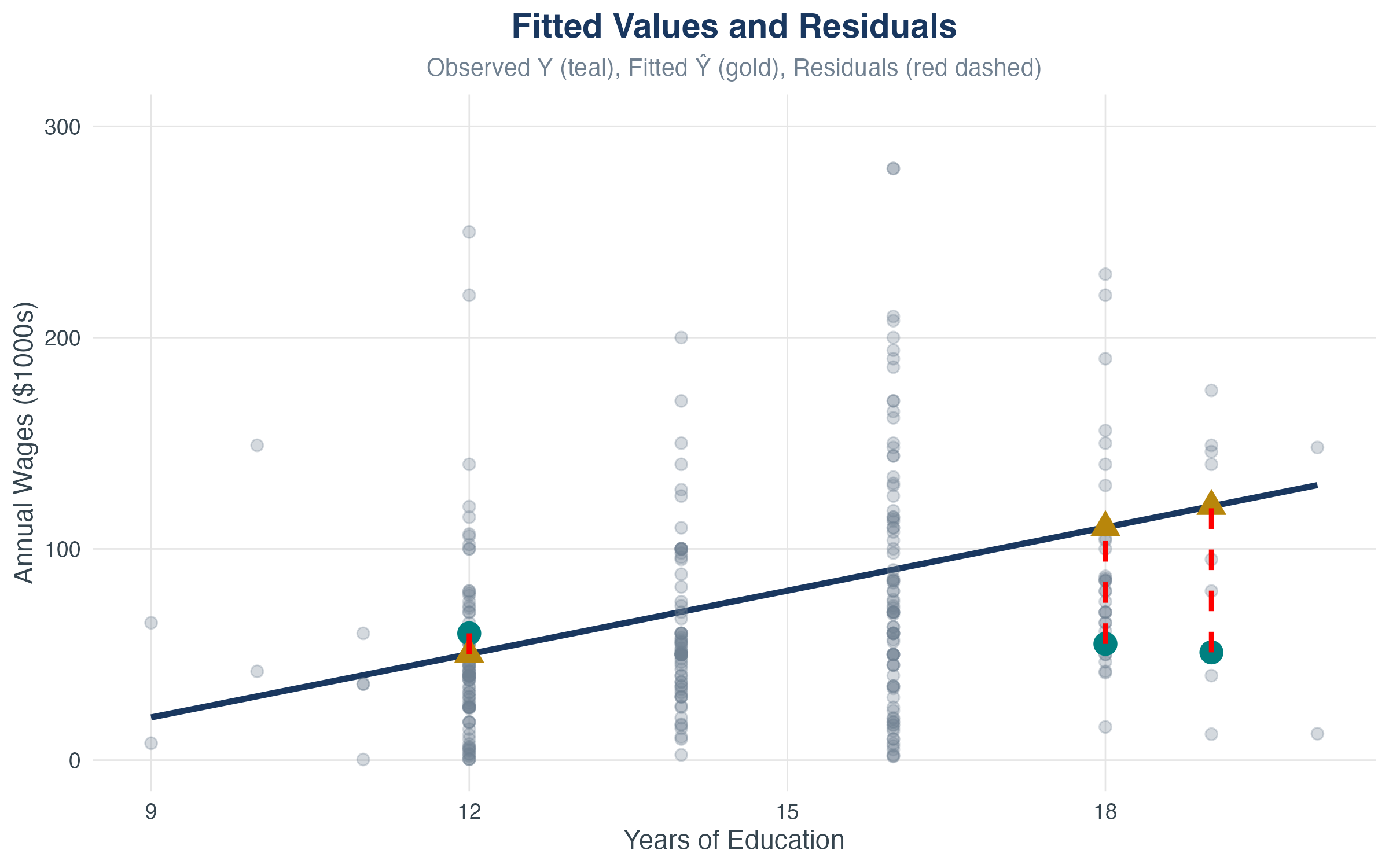
• Gold lines: residuals (vertical distance from point to line)
• OLS chooses the line that makes these distances smallest overall (in squared terms)

Stata: Running OLS Regression

Basic command:

regress wages education

Output includes:

• Coefficient estimates: \(\hat{\beta}_0\) (_cons) and \(\hat{\beta}_1\) (education)
• Standard errors (for inference - we’ll cover this later)
• R² (measure of fit)
• Number of observations

Generate fitted values and residuals:

predict wages_fitted, xb
predict residual, residuals

Reading Stata Regression Output

Understanding the table:

 Source | SS df MS Number of obs = 300
-------------+---------------------------------- F(1, 298) = 54.60
 Model | 298054 1 298054 Prob > F = 0.0000
 Residual | 1626752 298 5459.23 R-squared = 0.155
-------------+---------------------------------- Adj R-squared = 0.152
 Total | 1924806 299 6436.81 Root MSE = 73.883

------------------------------------------------------------------------------
 wages | Coef. Std. Err. t P>|t| [95% Conf. Interval]
-------------+----------------------------------------------------------------
 education | 13.022 1.762 7.39 0.000 9.552 16.492
 _cons | -114.740 25.633 -4.48 0.000 -165.187 -64.292
------------------------------------------------------------------------------

• Coef. column: \(\hat{\beta}_1 = 13.02\), \(\hat{\beta}_0 = -114.7\)
• R-squared: 0.155 (model explains 15.5% of variation)
• Root MSE: Standard error of regression (SER) = 73.88
• Std. Err.: We’ll use this for hypothesis tests (next chapter!)

Interpreting the Output

Example results: \[ \widehat{\text{Wages}} = -114.7 + 13.02 \cdot \text{Education}, \quad N = 300 \]

Interpretations:

• Slope (13.02): Each additional year of education is associated with approximately $13,020 more in annual wages
• Intercept (-114.7): Predicted wages when education = 0 (not meaningful here!)
• Predictions:
  • Person with 16 years of education: \(\hat{Y} = -114.7 + 13.02(16) = 93.6\)k
  • Person with 12 years of education: \(\hat{Y} = -114.7 + 13.02(12) = 41.5\)k
• Residual example: If someone with 12 years of education earns $35k, their residual is \(40 - 41.5 = -6.5\)k

Measuring How Well the Model Fits

Decomposing Variation

For any observation: \[ Y_i = \hat{Y}_i + \hat{u}_i \]

We can split total variation into two parts:

\[ \underbrace{Y_i - \bar{Y}}_{\text{Total deviation}} = \underbrace{\hat{Y}_i - \bar{Y}}_{\text{Explained deviation}} + \underbrace{\hat{u}_i}_{\text{Unexplained deviation}} \]

Squaring and summing across all observations:

\[ \underbrace{\sum_{i=1}^{n}(Y_i - \bar{Y})^2}_{\text{TSS}} = \underbrace{\sum_{i=1}^{n}(\hat{Y}_i - \bar{Y})^2}_{\text{ESS}} + \underbrace{\sum_{i=1}^{n}\hat{u}_i^2}_{\text{SSR}} \]

The Sum of Squares Trinity

Total Sum of Squares (TSS)

\[ TSS = \sum_{i=1}^{n}(Y_i - \bar{Y})^2 \] Measures total variation in \(Y\) around its mean.

Explained Sum of Squares (ESS)

\[ ESS = \sum_{i=1}^{n}(\hat{Y}_i - \bar{Y})^2 \] Variation in \(Y\) explained by the model (variation in fitted values).

Sum of Squared Residuals (SSR)

\[ SSR = \sum_{i=1}^{n}\hat{u}_i^2 \] Variation in \(Y\) not explained by the model (variation in residuals).

Why Does TSS = ESS + SSR? (The Algebra)

Start with the decomposition: \[ Y_i - \bar{Y} = (\hat{Y}_i - \bar{Y}) + (Y_i - \hat{Y}_i) \]

Square both sides: \[ (Y_i - \bar{Y})^2 = [(\hat{Y}_i - \bar{Y}) + (Y_i - \hat{Y}_i)]^2 \]

Expand: \[ (Y_i - \bar{Y})^2 = (\hat{Y}_i - \bar{Y})^2 + (Y_i - \hat{Y}_i)^2 + 2(\hat{Y}_i - \bar{Y})(Y_i - \hat{Y}_i) \]

Sum over all \(i\): \[ \sum_{i=1}^n (Y_i - \bar{Y})^2 = \sum_{i=1}^n (\hat{Y}_i - \bar{Y})^2 + \sum_{i=1}^n (Y_i - \hat{Y}_i)^2 + 2\sum_{i=1}^n (\hat{Y}_i - \bar{Y})(Y_i - \hat{Y}_i) \]

The cross-product term equals ZERO! (by properties of OLS) \[ TSS = ESS + SSR \]

Visualizing the Decomposition

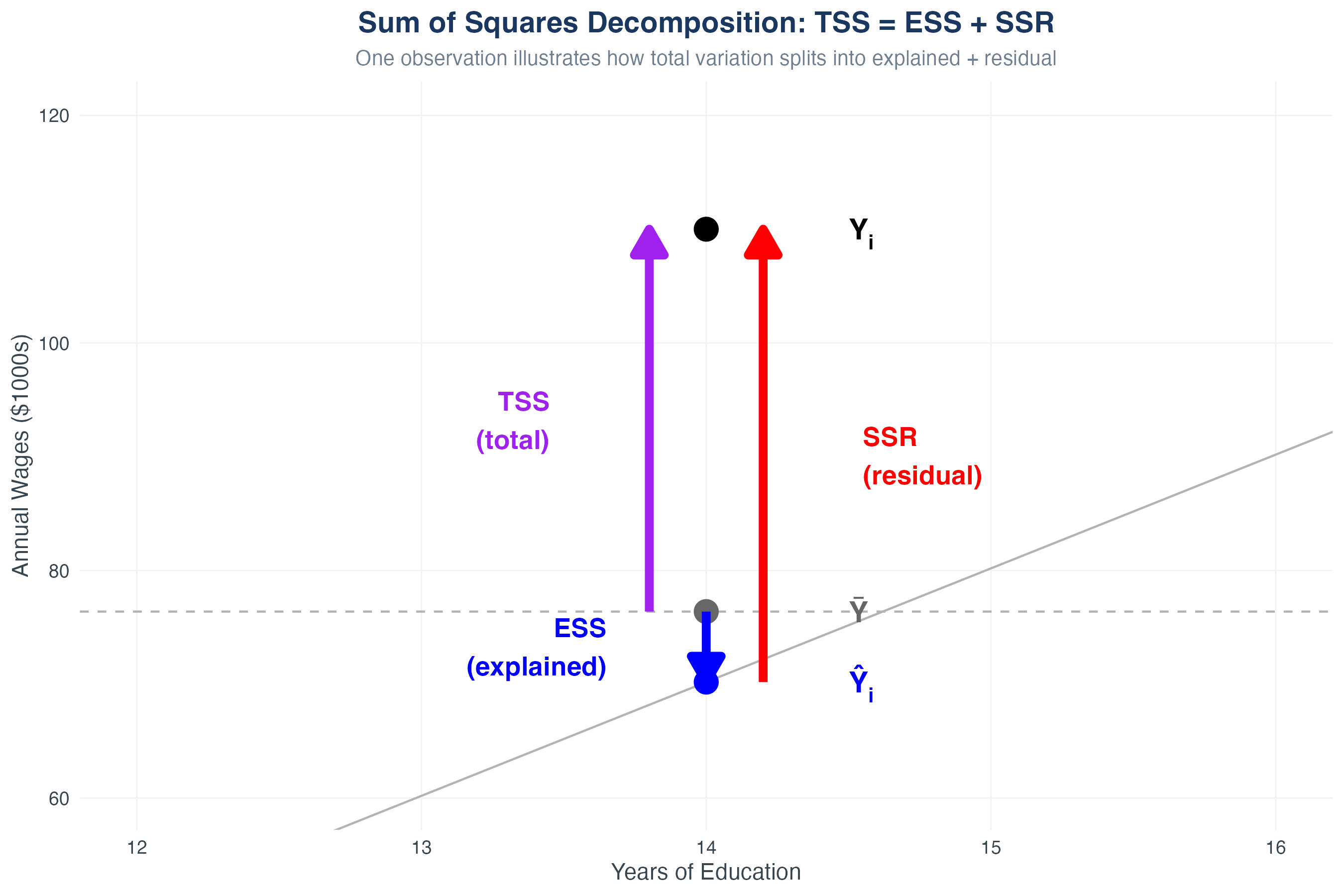
• Gray: Total deviation from mean (TSS)
• Blue: Explained by model (ESS)
• Gold: Unexplained residuals (SSR)

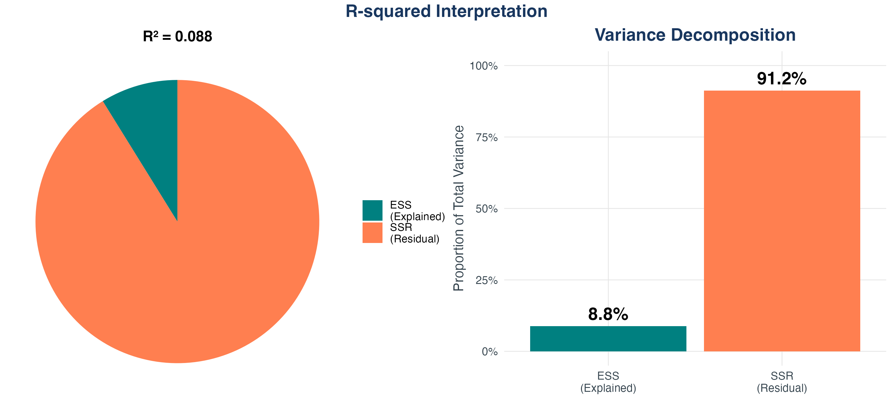
R-Squared: The Fraction Explained

\(R^2\) (R-squared)

\[ R^2 = \frac{ESS}{TSS} = 1 - \frac{SSR}{TSS} \]

Properties:

• \(0 \leq R^2 \leq 1\)

• \(R^2 = 0\): The model explains none of the variation (horizontal line at \(\bar{Y}\))

• \(R^2 = 1\): The model explains all variation (perfect fit, all points on the line)

• Typical values: \(R^2 = 0.10\) to \(0.30\) in social sciences (many factors matter!)

Critical Warning

A high \(R^2\) does not mean:

• The relationship is causal
• The model is correctly specified
• You have the “right” model

R-Squared Visualization

Standard Error of the Regression (SER)

How big are the typical residuals?

Standard Error of Regression

\[ SER = \sqrt{\frac{SSR}{n-2}} = \sqrt{\frac{\sum_{i=1}^{n}\hat{u}_i^2}{n-2}} \] Also called the “root mean squared error” (RMSE).

Interpretation:

• Measures typical size of prediction errors

• In original units of \(Y\) (unlike \(R^2\) which is unitless)

• Lower SER = better fit

• Divide by \(n-2\) (not \(n\)) because we estimated 2 parameters

Example: If SER = 7.9 in our education-wages regression, typical prediction error is about $7,900.

Assumptions for Unbiased Estimates

A Cautionary Tale: High R² \(\neq\) Unbiasedness

Provocative Example

Suppose we regress drowning deaths on ice cream sales: \[ \widehat{\text{Drownings}} = 2.1 + 0.003 \cdot \text{Ice Cream Sales} \]

R² = 0.89 (very high fit!)

Is this relationship meaningful, or just confounded?

\(\blacktriangleright\) No! Both are caused by a third factor: summer weather

• Hot days \(\Rightarrow\) more ice cream sales
• Hot days \(\Rightarrow\) more swimming \(\Rightarrow\) more drownings

The lesson: A model can fit the data well (high R²) but still yield biased estimates. This is why we need assumptions.

Unbiasedness: Getting the right answer

The Fundamental Question

We’ve estimated \(\hat{\beta}_1\), but is it correct? is \(\hat{\beta}_1\) an unbiased estimator of \(\beta_1\)?

Three least squares assumptions

Three key assumptions for unbiased OLS:

1. Zero conditional mean: \(E[u_i | X_i] = 0\)
   • Holds in RCT setting—we try to approximate this
   • Same as saying that \(u_i\) and X_i$ are uncorrelated . . .
2. i.i.d. sampling: \((X_i, Y_i)\) are independent and identically distributed

3. Finite fourth moments: Large outliers are unlikely (finite kurtosis)

Assumption 1: Zero Conditional Mean

Zero Conditional Mean

\[ E[u_i | X_i] = 0 \] The expected value of the error term is zero, after conditioning on \(X\).

• Both \(X\) and \(u\) have distributions in the population

• If, for example, \(X = education\), then we could (in principle) figure out its distribution in the population of adults

• Suppose (for simplicity), that \(u\) is ability (or age or gender or martial status, etc.). \(u\) will also have a distribution in the population

• So we are restricting how \(u\) and \(X\) relate to each other in the population

Simplifying assumption: \(E[u]=0\)

• First, we make a simplifying assumption without loss of generality:

\[E[u]=0\]

where \(E[\cdot]\) is the expected value operator

• Normalizing ability to be zero in the population should be harmless. It is.

Adjusting the intercept

• The presence of \(\beta_0\) in

\[Y = \beta_0 + \beta_1 X + u\]

allows us to assume that \(E[u] = 0\). If the average of \(u\) is different from zero, then we could jsut adjust the intercept, leaving the slope the same.

If \(\alpha_0 = E[u]\), then we can just add and subtract:

\[Y = (\beta_0 + \alpha_0) + \beta_1 X + (u-\alpha_0)\]

• New intercept is \(\beta_0 + \alpha_0\) Easy! But, our slope is unchanged.

Definition of simple regression model

KEY QUESTION: How do we need to restrict the dependence between \(u\) and \(X\)?

• We could assume that \(u\) and \(x\) are uncorrelated in the population:

\[Corr(X,u) = 0\]

• Zero correlation works for many purposes, but it only implies that \(u\) and \(X\) are not linearly related. Ruling out only linear dependence can cause problems with interpretation and makes analysis more difficult.

Definition of simple regression model

A better assumption involves the mean of the error term for each “slice” of the population determined by the values of X:

\[E[u|X] = E[u]\quad\text{for all values of }X \]

Where \(E[u|X]\) is “the expected value of \(u\) given \(X\).”

• We say that \(u\) is mean independent of x.

• How realistic is this?

Definition of simple regression model

Suppose that \(u\) is “ability” and \(X\) is years of education. Then we need, for example:

\[E[ability|X = 8] = E[ability|X = 12] = E[ability|X = 16]\]

The average ability is the same in different portions of the population with an 8th grade education, 12th grad education, and four-year college education.

Zero conditional mean assumption.

• When we combine this assumption with our normalization (\(E[u]=0\)), then we get

\[E[u|X] = 0 \quad \text{for all values of }X\]

• And this is the zero conditional mean assumption

This is the KEY assumption

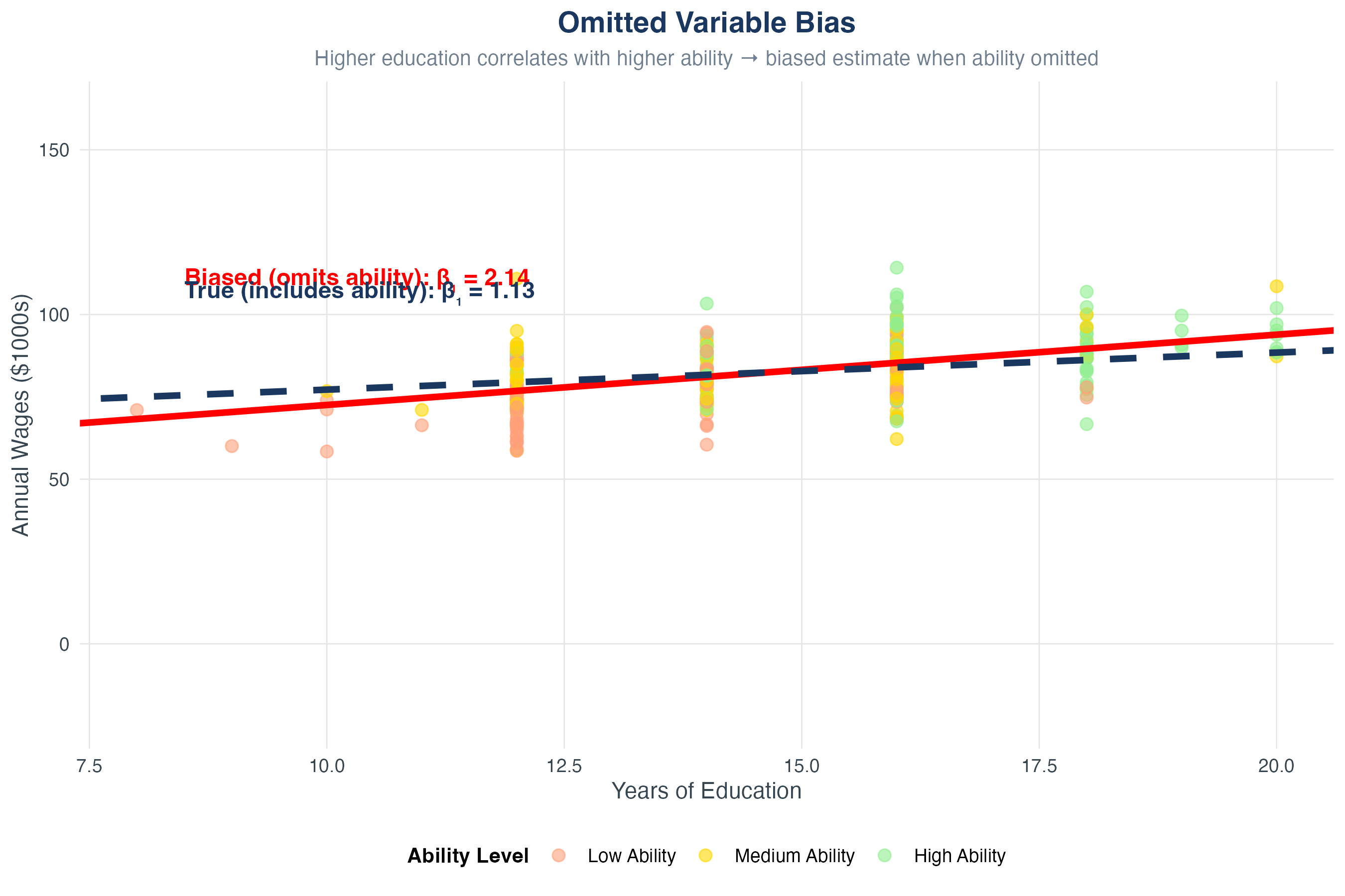
If \(E[u|X] \neq 0\), then \(\hat{\beta}_1\) is biased — it systematically estimates the wrong thing.

This is called omitted variable bias.

Visualizing Zero Conditional Mean

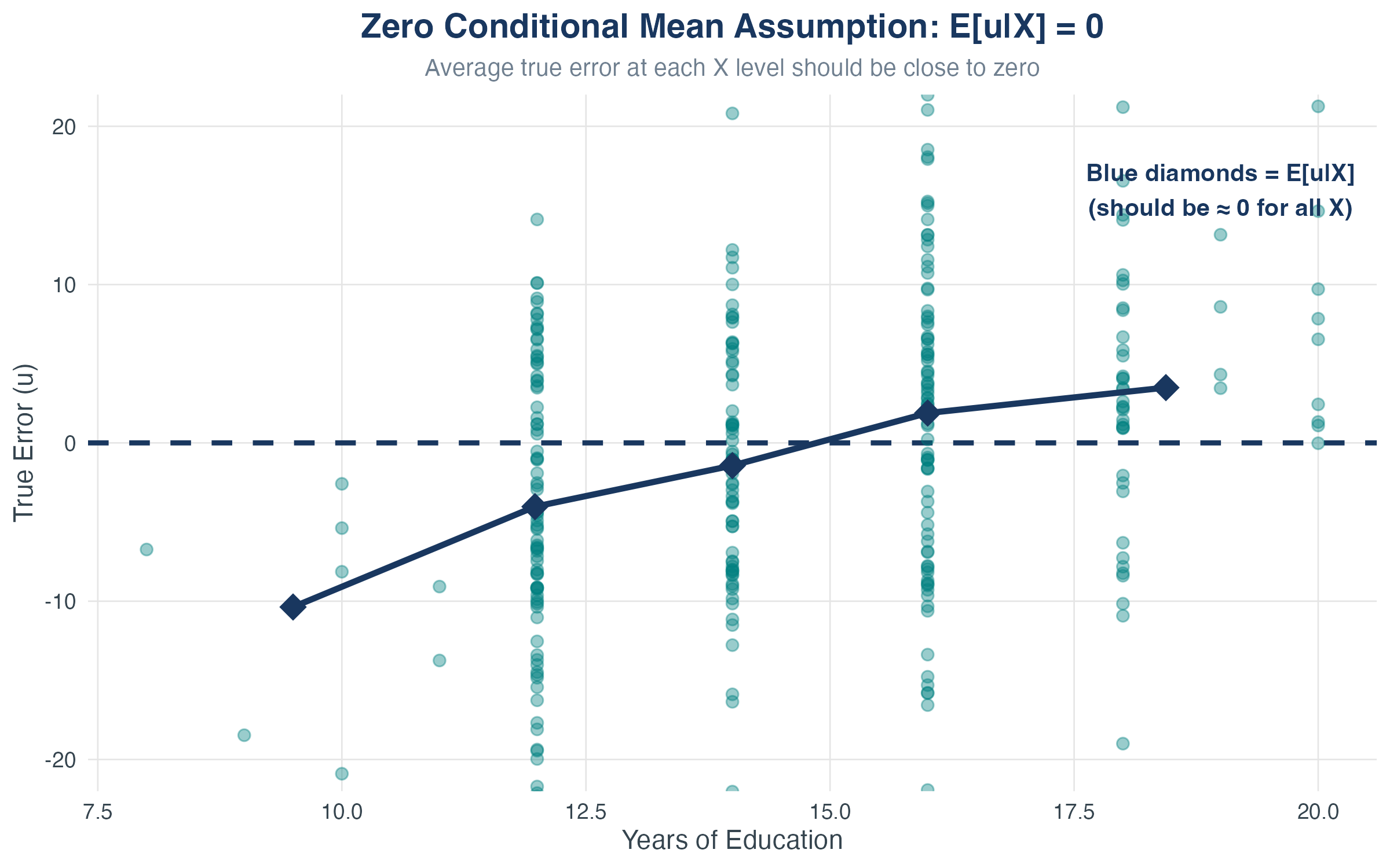
What this shows:

• Residuals (teal points) are evenly scattered above and below zero
• Red diamonds show the average residual at each education level: \(E[u|X]\)

Zero conditional mean assumption

Because the expected value is a linear operator, then \(E[u|X] = 0\) implies that

\[E[Y|X] = \beta_0 + \beta_1 X + E[u|X] = \beta_0 + \beta_1 X\]

This shows that the population regression function is a linear function of X!

Nice.

When Does Zero Conditional Mean Fail?

Example: Education and wages \[ \text{Wage} = \beta_0 + \beta_1 \cdot \text{Education} + u \]

What’s in \(u\)?

• Ability, motivation, family background, connections

Problem:

• High-ability people tend to get more education

• So \(E[u | \text{Education = high}]\) > \(E[u | \text{Education = low}]\)

• Violates zero conditional mean!

• Result: \(\hat{\beta}_1\) overestimates the causal effect of education (it picks up both education and ability)

Omitted Variable Bias (OVB)

Sampling Distributions and Uncertainty

\(\hat{\beta}_1\) is a Random Variable

Key insight: Our estimates \(\hat{\beta}_0\) and \(\hat{\beta}_1\) depend on the sample.

• Different samples \(\Rightarrow\) different estimates

• If we drew a new sample, we’d get a different \(\hat{\beta}_1\)

• This creates a sampling distribution

Under the three assumptions:

• \(\hat{\beta}_1\) is unbiased: \(E[\hat{\beta}_1] = \beta_1\)

• \(\hat{\beta}_1\) is consistent: As \(n \to \infty\), \(\hat{\beta}_1 \to \beta_1\)

• By the CLT, \(\hat{\beta}_1\) is approximately normal for large \(n\)

  • Usually, we are quite happy with \(n > 100\)

Sampling Distribution Visualization

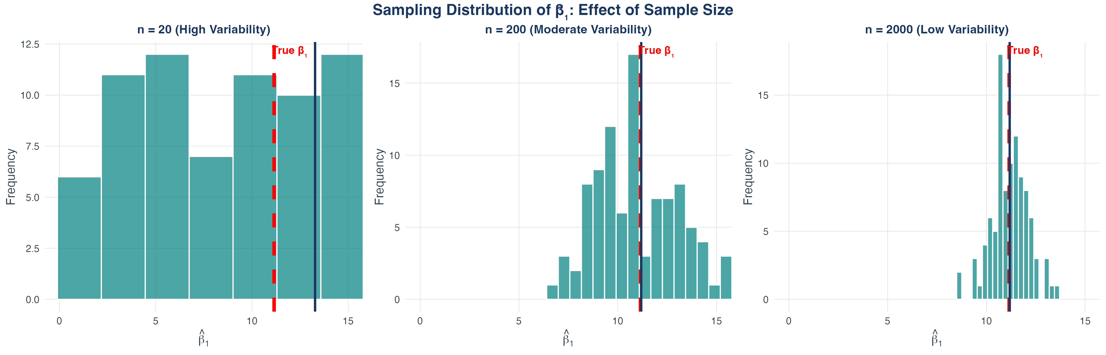
• 1,000 different samples, each with \(n = 300\)
• Each sample gives a different \(\hat{\beta}_1\)
• Mean of estimates equals true \(\beta_1\) (unbiased!)
• Larger \(n\) \(\Rightarrow\) tighter distribution (more precise)

Effect of Sample Size on Precision

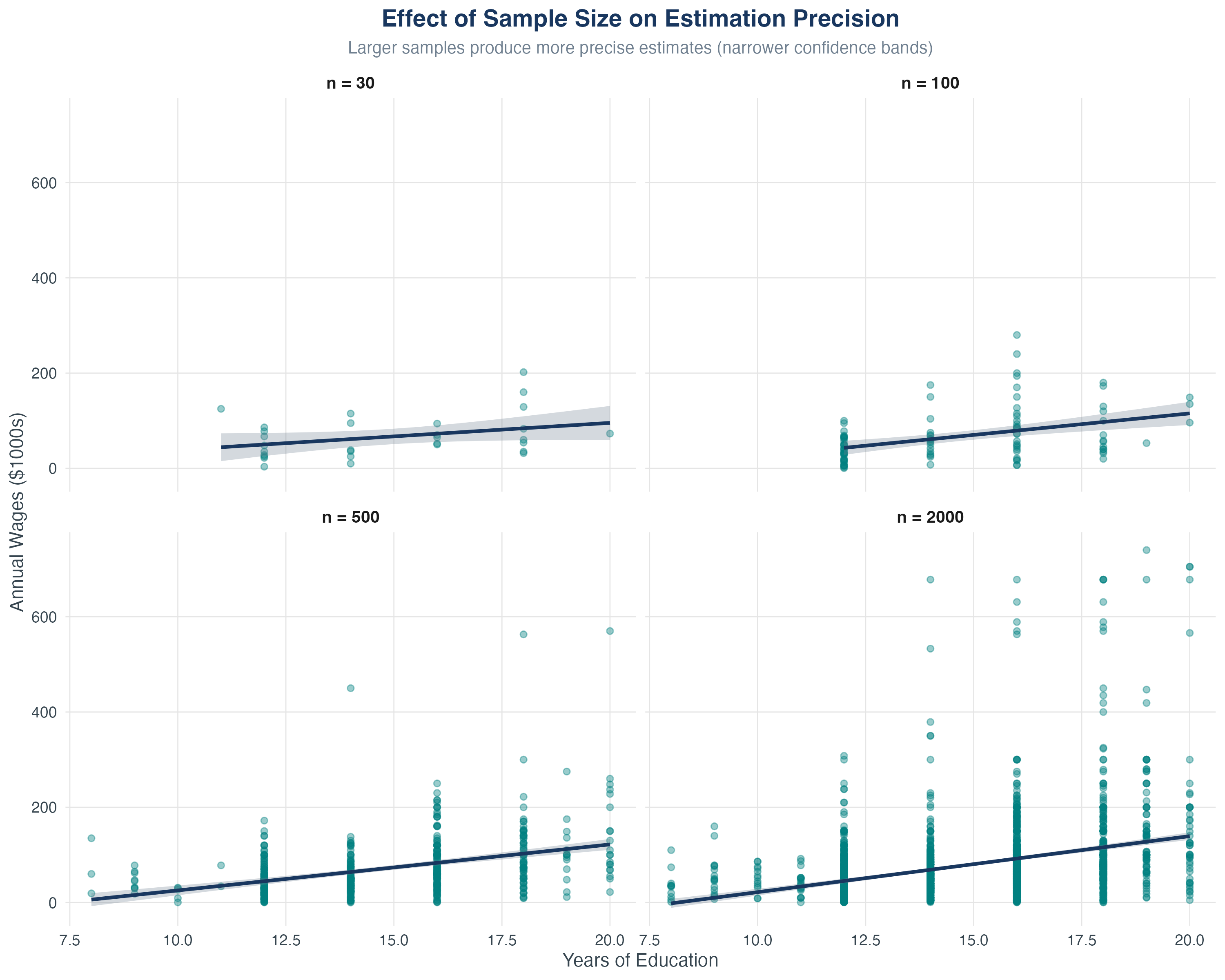
Key takeaway: Larger samples give more precise estimates (tighter confidence bands).

What Determines the Variance of \(\hat{\beta}_1\)?

The variance of \(\hat{\beta}_1\) is: \[ \sigma^2_{\hat{\beta}_1} = \frac{1}{n} \frac{\operatorname{Var}\!\left[(X_i - \mu_X) u_i\right]} {\operatorname{Var}(X_i)^2} \]

Interpretation:

• Larger \(n\): More data \(\Rightarrow\) smaller variance (more precise)

• Larger \(\text{Var}(X)\): More spread in \(X\) \(\Rightarrow\) smaller variance (easier to detect slope)

• Larger \(\sigma^2_u\): Noisier errors \(\Rightarrow\) larger variance (harder to estimate)

\(\blacktriangleright\) We’ll use this in the next chapter for hypothesis testing and confidence intervals.

Bringing It All Together

The Big Picture

Key Takeaways

1. We minimize the sum of squared residuations to estimate \(\beta_1\) and \(\beta_0\)
2. Slopes have precise interpretations: \(\Delta Y\) per unit \(\Delta X\), holding \(u\) fixed
3. \(R^2\) and SER measure model fit, but don’t relate to causality
4. Zero conditional mean is THE critical assumption for unbiased estimation
5. \(\hat{\beta}_1\) has a sampling distribution — it’s random, not fixed
6. Larger samples and more variation in \(X\) give more precise estimates

Next chapter: Hypothesis testing and confidence intervals — how to make formal inferences about \(\beta_1\).

Bonus: Common Misconceptions and Clarifications

Misconception #1: “Correlation = Causation”

Misconception

“Education and wages are correlated, so education causes higher wages.”

Clarification

Regression shows association, not necessarily causation.

• Could be reverse causality (higher earners invest more in education)

• Could be omitted variable bias (ability affects both)

• Need experimental or quasi-experimental design for causal claims

Key point: OLS estimates the conditional expectation E[Y|X], not a causal effect.

Misconception #2: “High R² = Good Model”

Misconception

“R² = 0.30 is low, so this is a bad model.”

Clarification

R² depends on the context!

• In physics: R² > 0.95 is common (physical laws are precise)

• In social sciences: R² = 0.30 can be excellent (human behavior is complex)

• R² measures explained variance, not model validity

Better questions:

• Are coefficients statistically significant?
• Do they have the expected signs?
• Are residuals well-behaved?

Misconception #3: “Intercept Must Be Meaningful”

Misconception

“\(\beta_0\) = -114.7 means someone with zero education earns -$114,700? That’s impossible!”

Clarification

The intercept is often not interpretable in practice.

• It’s the predicted Y when X = 0

• But X = 0 may be outside the range of data (no one has 0 years of education)

• It’s an extrapolation, not an actual prediction

Key point: The intercept ensures the regression line passes through \((\bar{X}, \bar{Y})\) - it’s a technical parameter, not always economically meaningful.

Misconception #4: “Residuals = Errors”

Misconception

“The residual \(\hat{u}_i\) is the same as the true error \(u_i\).”

Clarification

They are different (and we never observe \(u_i\)!):

• Error \(u_i = Y_i - (\beta_0 + \beta_1 X_i)\) (population, unknown)

• Residual \(\hat{u}_i = Y_i - (\hat{\beta}_0 + \hat{\beta}_1 X_i)\) (sample, observed)

Relationship: Residuals estimate errors, but they’re not identical. \[ \hat{u}_i = u_i - (\hat{\beta}_0 - \beta_0) - (\hat{\beta}_1 - \beta_1)X_i \]

Misconception #5: “Adding X Always Helps”

Misconception

“More variables = better model, always.”

Clarification

Only add variables that belong in the model:

• Irrelevant variables increase standard errors (reduce precision)

• Can lead to multicollinearity problems

• Overfitting: model fits sample noise, not population relationship

Principle: Use theory to guide variable selection, not just R².

Bonus: Implementing OLS in Stata

Complete Stata Workflow

Full analysis in Stata:

* Load data
import delimited "education_wages_data.csv", clear

* Summary statistics
summarize education wages

* Scatter plot
scatter wages education

* Correlation
correlate education wages

* Run OLS regression
regress wages education

* Generate fitted values and residuals
predict wages_fitted, xb
predict residual, residuals

* Check sum of residuals
summarize residual

Calculating Fit Statistics in Stata (Part 1)

Calculate TSS, ESS, and SSR manually:

* After running: regress wages education
* Store basic stats from regression
scalar r2 = e(r2)
scalar ser = e(rmse)
scalar n = e(N)

* Calculate mean of Y
quietly sum wages
scalar y_bar = r(mean)

* Generate squared deviations
gen deviation_total = (wages - y_bar)^2
gen deviation_explained = (wages_fitted - y_bar)^2
gen deviation_residual = residual^2

What we’re doing: Creating three variables to capture total, explained, and unexplained variation.

Calculating Fit Statistics in Stata (Part 2)

Sum up and verify the decomposition:

* Sum the squared deviations
quietly sum deviation_total
scalar TSS = r(sum)

quietly sum deviation_explained
scalar ESS = r(sum)

quietly sum deviation_residual
scalar SSR = r(sum)

* Verify: TSS = ESS + SSR
display "TSS = " TSS
display "ESS = " ESS
display "SSR = " SSR
display "Check: TSS - (ESS + SSR) = " (TSS - (ESS + SSR))

Interpretation: The check should equal zero (or very close), confirming \(TSS = ESS + SSR\).

Practice & Resources

Recommended practice:

• Stock & Watson Chapter 4 odd-numbered exercises
• Beyond our lab, practice running and interpreting regressions on the ACS data
• Practice interpreting coefficients out loud

Next session: Hypothesis testing, \(t\)-statistics, and confidence intervals