Instrumental Variables

SW Chapter 12

ECON3500: Econometrics and Applications

Spring 2026

Learning Objectives

1. Understand why we need instrumental variables to address endogeneity
2. Identify the three key characteristics of a valid instrument
3. Explain the mechanics of two-stage least squares (2SLS)
4. Test for weak instruments using first-stage F-statistics
5. Combine IV with panel data and fixed effects

Textbook Coverage

• 12.1: IV estimator with single regressor and single instrument
  • We won’t manually compute standard errors
• 12.2: General IV regression model
• 12.3: Checking instrument validity
  • Weak instruments and exogeneity
  • Exclude overidentifying restrictions test
• 12.4/12.5: Interesting examples!

Why Instrumental Variables?

The Endogeneity Problem

Three threats to internal validity all produce endogeneity—the regression \(X_i\) is correlated with the error term. That is, \(E(u_i | X_i) \neq 0\):

1. Omitted variable bias: An unobserved variable correlated with \(X\) is left out

2. Simultaneous causality: \(X\) causes \(Y\), but \(Y\) also causes \(X\)

3. Errors-in-variables bias: \(X\) is measured with error

What We’ve Tried So Far

Solutions to endogeneity considered previously:

• Difference-in-differences
  • Requires a clear before/after treatment
• Fixed effects (Ch. 10)
  • Requires panel data
  • Endogeneity source must be time-constant
  • Regressors must not be time-constant

Today: Instrumental variables (IV)

• Widely-used method for addressing endogeneity
• IV can eliminate bias when \(E(u_i | X_i) \neq 0\) if we have a valid instrumental variable \(Z\)

Wages and Schooling

\[\log(wage_i) = \beta_0 + \beta_1 schooling_i + \delta V_i + u_i\]

• \(\beta_1\) measures the returns to schooling
• One omitted variable \(V\): innate ability as a worker
  • Innate ability positively affects wages (\(\delta > 0\))
  • Likely that innate ability is positively correlated with schooling: \(\text{corr}(schooling, V) > 0\)

• OLS estimator of \(\beta_1\) may have omitted variable bias
• If this is the only omitted variable, bias is positive
  • \(\hat{\beta}_1\) overestimates the financial returns to schooling

Can We Fix This with Multiple Regression?

\[\log(wage_i) = \beta_0 + \beta_1 schooling_i + \delta V_i + u_i\]

• How do we measure innate ability?

• IQ tests may capture some part of ability; hard to get IQ data for large samples

• IQ is not a perfect measure of innate ability in the workplace
  • Example: IQ tests wouldn’t measure social skills
  • Note: you should include IQ or equivalent if available

• Since IQ tests are imperfect, schooling likely remains correlated with the omitted part of innate ability

• Multiple regression doesn’t fully solve this problem!

Can We Fix This with Panel Data?

\[\log(wage_i) = \beta_0 + \beta_1 schooling_i + \delta V_i + a_i + u_i\]

• Innate ability might be reasonably constant over a career, captured by \(a_i\)
• But schooling is also typically constant for adult workers

• Adults who go back to school after working are a non-representative group
• Panel data do not provide convincing variation in schooling over a worker’s career
• Fixed effects won’t work here! (and if they do, won’t capture the type of variation we care about)

Bottom Line

Neither multiple regression nor panel data convincingly addresses the ability bias in estimating returns to schooling. We need a different approach.

Endogeneity as a DAG

The Problem in a DAG

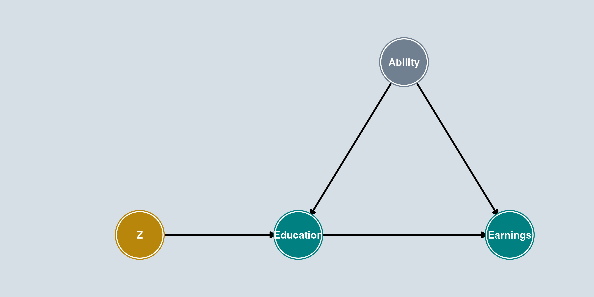
To understand how IV solves this, let’s visualize the problem using causal diagrams from Ch 8b.

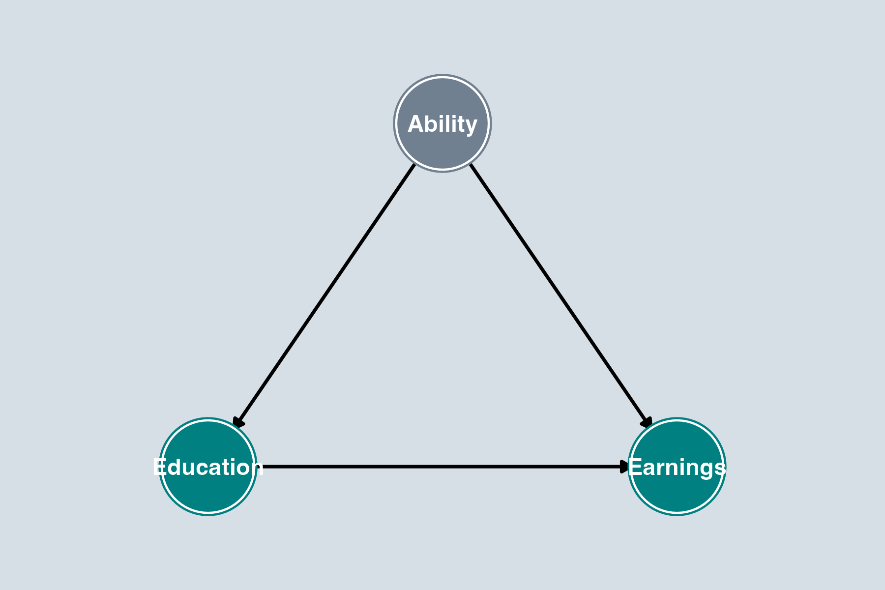
Gray = unobserved

From Ch 8b, we know this DAG:

• Causal path: Education → Earnings ✓
• Backdoor path: Education ← Ability → Earnings ✗

The backdoor path is open and Ability is unobserved.

• Can’t control for it (Ch 6/7)
• Can’t difference it out (Ch 10)
• We need a new tool to close this path.

The IV Solution in a DAG

Gold = instrument, Gray = unobserved

Add an instrument \(Z\) to the DAG. A valid instrument must satisfy:

1. Z → Education: \(Z\) affects \(X\) (relevance)
2. No Z ← Ability: \(Z\) is not connected to unobserved confounders (exogeneity)
3. No Z → Earnings: \(Z\) does not directly affect \(Y\) (exclusion)

Key Insight

IV works by isolating the variation in Education that comes only from \(Z\). Since \(Z\) has no connection to Ability and no direct effect on Earnings, this variation is “clean” — free of confounding.

Cigarette Demand: A Running Example

Demand for Cigarettes

Broad public policy interest in reducing cigarette consumption.

\[sales_i = \beta_0 + \beta_1 price_i + u_i\]

• Price may be correlated with omitted variables in \(u\): firms set prices based on demand conditions
• When state \(i\) has unusually high demand (\(u_i\) high), prices are higher too
• This is simultaneous causality: sales depend on prices, but prices also depend on sales

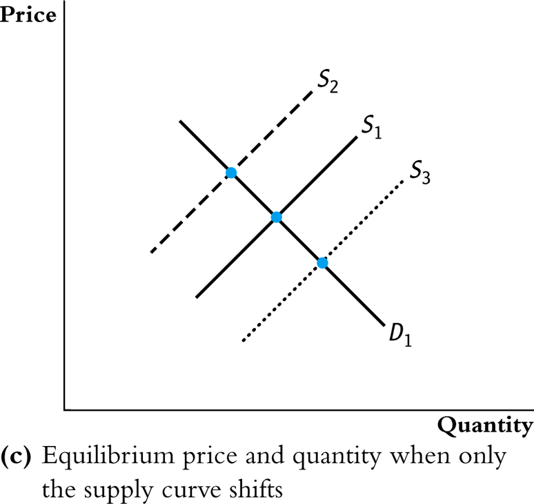
The identification problem: When both supply and demand shift, equilibrium data trace out neither curve — just a scatter of equilibrium points.

We need something that shifts supply without shifting demand.

The IV Intuition

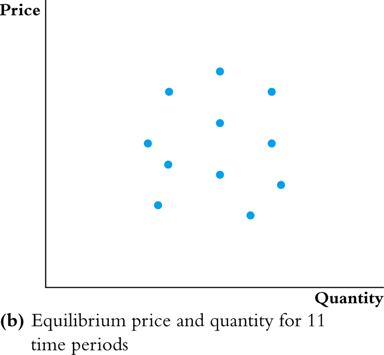
If we can hold demand fixed and only observe supply shifting:

• The equilibrium points trace out the demand curve
• The instrument shifts supply without directly affecting demand — it moves \(X\) without directly affecting \(Y\)

Why Simultaneous Causality Is Especially Problematic

\[sales_i = 164.4 - 0.38 \cdot price_i + u_i\]

• Simultaneous causality is especially problematic because \(X_i\) will generally be correlated with all omitted variables in \(u_i\)
• Hard to remove OVB by measuring the omitted variables
• Would need to measure every single omitted variable

Simultaneous causality would disappear if we could randomly assign prices to the different states

• In that experiment, there would be no correlation between price and \(u\)
• IV provides a way to mimic this

The IV Solution: Formal Definitions

Instrumental Variables: Three Assumptions

We introduced these conditions visually using DAGs. Now let’s state them formally.

An instrumental variable is an additional variable \(Z_i\) that satisfies three assumptions:

1. \(Z_i\) is correlated with \(X_i\)
   • \(\text{Corr}(Z, X) \neq 0\)
   • \(Z\) is a powerful or relevant instrument

2. \(Z_i\) is not correlated with the omitted variable, \(u_i\)
   • \(\text{Corr}(Z, u) = 0\)
   • \(Z\) is an exogenous instrument

3. \(Z_i\) does not directly affect (cause) \(Y_i\)
   • It can only affect \(Y_i\) through its effect on \(X_i\)
   • \(Z\) is an excluded instrument
   • \(Z_i\) does not enter the equation \(Y_i = \beta_0 + \beta_1 X_i + u_i\)

Two vs. Three Assumptions

Some textbooks combine (2) and (3) into a single validity or exogeneity condition: \(\text{Corr}(Z, u) = 0\). Others (including SW) separate them: exogeneity (Z uncorrelated with \(u\)) and exclusion (Z affects Y only through X). The practical question is the same either way: can Z affect Y through any channel other than X?

The Wald Estimator

With a binary instrument \(Z_i \in \{0, 1\}\), there is a simple way to see how IV works:

First stage: How does \(Z\) move \(X\)?

\[\text{First stage} = E[X_i \mid Z_i = 1] - E[X_i \mid Z_i = 0]\]

Reduced form: How does \(Z\) move \(Y\)?

\[\text{Reduced form} = E[Y_i \mid Z_i = 1] - E[Y_i \mid Z_i = 0]\]

\[\boxed{\hat{\beta}_1^{Wald} = \frac{\text{Reduced form}}{\text{First stage}}}\]

Intuition

The reduced form tells us how the instrument changes the outcome. The first stage tells us how the instrument changes treatment. Their ratio tells us the effect of treatment induced by the instrument.

Identification

Start with the population model:

\[Y = \beta_0 + \beta_1 X + u\]

Take the covariance of both sides with \(Z\):

\[\text{Cov}(Y, Z) = \text{Cov}(\beta_0 + \beta_1 X + u, Z)\] \[= \text{Cov}(\beta_0, Z) + \text{Cov}(\beta_1 X, Z) + \text{Cov}(u, Z)\] \[= 0 + \beta_1 \text{Cov}(X, Z) + 0 \quad \text{by } \text{Cov}(u, Z) = 0\]

Solving for \(\beta_1\):

\[\boxed{\beta_1 = \frac{\text{Cov}(Y, Z)}{\text{Cov}(X, Z)}}\]

Which Assumptions Did We Use?

\[\beta_1 = \frac{\text{Cov}(Y, Z)}{\text{Cov}(X, Z)}\]

• \(\text{Cov}(Z_i, u_i) = 0\) — explicitly used in the derivation
• \(\text{Cov}(X_i, Z_i) \neq 0\) — used to divide by \(\text{Cov}(X, Z)\); can’t divide by zero!
• \(Z_i\) does not affect \(Y_i\) directly — used to write the population model as \(Y_i = \beta_0 + \beta_1 X_i + u_i\)

Key Feature of IV

Notice we never assumed \(\text{Cov}(X_i, u_i) = 0\). IV explicitly allows for endogeneity — that’s the whole point!

Intuition for the IV Formula

\[\beta_1 = \frac{\text{Cov}(Y, Z)}{\text{Cov}(X, Z)}\]

• Goal: estimate \(\beta_1\), how \(X\) affects \(Y\)
• Problem: We think \(X\) is correlated with \(u\)
• Solution: Don’t compare \(Y\) (which contains \(u\)) and \(X\) directly
  • \(\text{Cov}(X, Y)\) is explicitly not in our formula

• Instead, see how \(Y\) moves with a third variable \(Z\), and how \(X\) moves with \(Z\)
• \(Z\) is exogenous: uncorrelated with \(u\); \(Z\) also does not affect \(Y\) directly
• If \(Y\) and \(X\) are both correlated with \(Z\), the only explanation under our assumptions is that \(X\) causes \(Y\) according to \(\beta_1\)

Applying the Formula: Distance to College

Back to our wages/schooling example. Instrument: distance from childhood home to nearest college.

\[\beta_1 = \frac{\text{Cov}(\log \text{wage}, \text{distance})}{\text{Cov}(\text{schooling}, \text{distance})}\]

• Denominator is positive (closer to college → more schooling)
• Numerator is positive if people near a college earn higher wages as adults
• Note: not because the distance causes the higher wage

Key Feature

\(\text{Cov}(X, Y)\) does not appear in the formula — we never directly compare someone’s wage to their schooling. Instead, we use only the variation in schooling driven by distance.

Two-Stage Least Squares

The 2SLS Estimator

For a dataset with \(n\) observations, replace population covariances with sample covariances:

\[\hat{\beta}_1^{2SLS} = \frac{\widehat{\text{Cov}}(Y, Z)}{\widehat{\text{Cov}}(X, Z)} = \frac{\frac{1}{n}\sum_{i=1}^{n}(Y_i - \bar{Y})(Z_i - \bar{Z})}{\frac{1}{n}\sum_{i=1}^{n}(X_i - \bar{X})(Z_i - \bar{Z})}\]

\[\hat{\beta}_0^{2SLS} = \bar{Y} - \hat{\beta}_1^{2SLS}\bar{X}\]

Called two-stage least squares — why will become apparent shortly.

What Are the Two Stages?

Stage 1: Regress \(X\) on \(Z\) (the “first stage”)

\[X_i = \pi_0 + \pi_1 Z_i + v_i\]

Form the predicted values:

\[\hat{X}_i = \hat{\pi}_0 + \hat{\pi}_1 Z_i\]

Note: \(X_i = \color{green}{\hat{X}_i} + \color{red}{\hat{v}_i}\)

Stage 2: Regress \(Y\) on \(\hat{X}\) (the “second stage”)

\[Y_i = \beta_0 + \beta_1 \hat{X}_i + u_i\]

Intuition: Why 2SLS Works

• First stage regresses \(X\) on \(Z\)
  • Forms a “best guess” of \(X\) using only data on \(Z\)
• The predicted \(\hat{X}\) is not correlated with omitted variables in the second stage
  • If we predict price using sales tax, predicted prices can’t be correlated with unmeasured factors that affect demand
  • We assumed exogeneity: sales tax is uncorrelated with omitted variables

• Second stage regresses \(Y\) on \(\hat{X}\)
  • \(\hat{X}\) is “cleansed” of any correlation with omitted variables
  • No more OVB or simultaneous causality bias

Key Insight

The instrument isolates the variation in \(X\) that is exogenous. 2SLS uses only this “clean” variation to estimate \(\beta_1\).

The Local Average Treatment Effect

IV uses only the variation in \(X\) driven by the instrument — that’s the whole point.

But this also means we can only observe the effect among people for whom the instrument actually affects their treatment.

• Suppose a treatment improves your outcome by 2, but my outcome by only 1
• And the instrument strongly affects whether you get treatment, but barely affects me
• Then the IV estimate will be much closer to 2 than to 1

Local Average Treatment Effect (LATE)

The IV estimate is local to the people whose treatment status is changed by the instrument, weighted by how much the instrument affects them. It is not the average effect for all units, or even for all treated units.

Better LATE Than Never?

Implication: The IV estimate may not represent the average effect for everyone — or even for those actually treated.

• Compared to a randomized experiment, IV may be less informative about what would happen if treatment were expanded to a broader population

• But IV still provides a valid causal estimate for the subgroup whose behavior is changed by the instrument
• When exogenous variation is limited, LATE may be the best causal estimate available

Practical Implication

When interpreting IV results, ask: For whom does the instrument induce treatment? The IV estimate applies to that group — not necessarily to all units in the sample.

Cigarette Demand: IV in Practice

The Instrument: Sales Tax

\[sales_i = \beta_0 + \beta_1 price_i + u_i\]

• Instrument for price of cigarettes? Need a \(Z_i\) that is:
  • Powerful: Correlated with price
  • Exogenous: Uncorrelated with \(u_i\) (unobserved demand factors)
  • Excluded: Does not directly impact cigarette demand

• Sales tax in state \(i\)?
  • Powerful: Sales tax should be positively correlated with price (price measured inclusive of taxes)
  • Exogenous: Plausible, but contestable: states with stronger anti-smoking preferences may both set higher taxes and have lower cigarette demand
  • Excluded: Plausible, but contestable: the tax affects demand primarily through price, not through other channels

2SLS in Stata

Stata’s ivregress command handles both stages automatically:

ivregress 2sls packpc (avgprs=tax), robust

ivregress 2sls Y (X=Z), robust

• \(Y\) = dependent variable (first after 2sls)
• \(X\) = endogenous regressor (in parentheses before =)
• \(Z\) = excluded instrument (after =)
• robust = heteroskedasticity-robust standard errors

Stata: 2SLS Results

. ivregress 2sls packpc (avgprs=tax), robust

Instrumental variables (2SLS) regression Number of obs = 96
 Wald chi2(1) = 88.46
 Prob > chi2 = 0.0000
 R-squared = 0.4219
 Root MSE = 19.567

------------------------------------------------------------------------------
 | Robust
 packpc | Coefficient std. err. z P>|z| [95% conf. interval]
-------------+----------------------------------------------------------------
 avgprs | -.4208748 .0447474 -9.41 0.000 -.5085781 -.3331715
 _cons | 169.556 7.516482 22.56 0.000 154.824 184.2881
------------------------------------------------------------------------------
Instrumented: avgprs
Instruments: tax

2SLS estimates that a 1-unit increase in price leads to a decrease of 0.42 packs per capita.

Viewing Both Stages with first

ivregress 2sls packpc (avgprs=tax), robust first

The first option displays the first-stage regression alongside the second stage.

Reporting the First Stage

• First stage shows how \(X\) and \(Z\) are related
• It provides a statistical test of the relevance assumption: \(\text{Corr}(X, Z) \neq 0\)

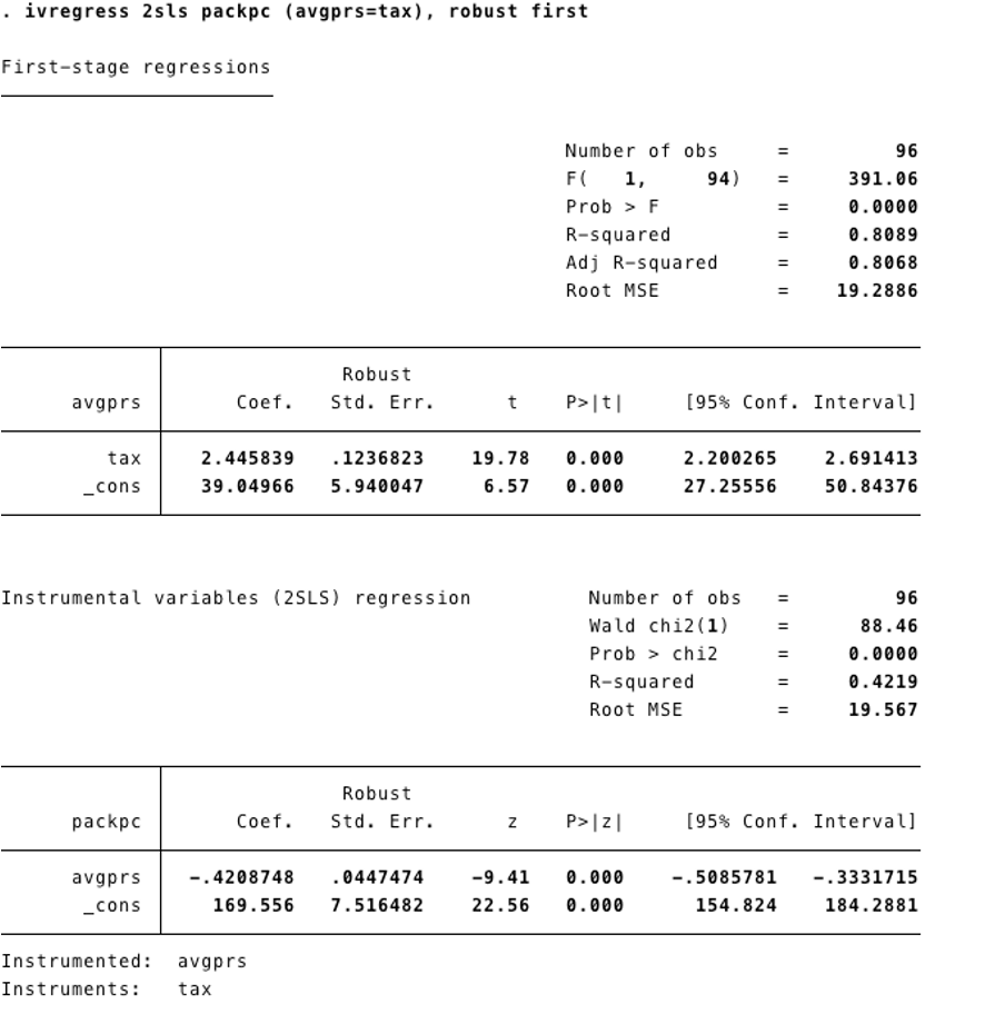
Rule of Thumb: F > 10

A common rule of thumb is that the first-stage F-statistic should be greater than 10. If so, instruments are likely powerful (relevant). This threshold is a guide, not a bright line.

Checking Instrument Validity

Weak Instruments

What if the first-stage F-test is less than 10?

• May have a weak instrument
• Sample covariance of \(X\) and \(Z\) may be close to 0

\[\hat{\beta}_1^{2SLS} = \frac{\widehat{\text{Cov}}(Y, Z)}{\widehat{\text{Cov}}(X, Z)}\]

• Intuition: dividing by something close to zero blows up your estimate
• Large standard errors and unreliable point estimates

Consequences of Weak Instruments

If the first-stage F-statistic is less than 10, the 2SLS estimates may be biased and confidence intervals may have incorrect coverage. Do not trust the results.

Which Assumptions Can Be Tested?

Assumption	Testable?	How?
Relevance (\(\text{Corr}(Z, X) \neq 0\))	Yes	First-stage F-test (rule of thumb: > 10)
Exogeneity (\(\text{Corr}(Z, u) = 0\))	No	Must argue based on institutional knowledge
Exclusion (\(Z\) doesn’t directly cause \(Y\))	No	Must argue based on theory

Exogeneity and Exclusion Cannot Be Tested

You lack data on the omitted variable, so you cannot test whether \(Z\) is correlated with it. Both exogeneity and exclusion must be defended with reasoning — relevance is the only one with a formal test.

IV with Multiple Regressors

Adding Exogenous Controls

\[sales_i = \beta_0 + \beta_1 price_i + \beta_2 income_i + u_i\]

• Income per person at the state level may affect cigarette sales
• Income is not determined simultaneously with cigarette demand
  • We assume income is uncorrelated with the composite error \(u\)

• 2SLS can handle variables not treated as endogenous
• Income enters both stages:
  • First stage: helps predict price
  • Second stage: controls for income’s direct effect on sales

ivregress 2sls packpc (avgprs=tax) incomepop, robust first

Need an Excluded Instrument

• We need at least one instrument for each regressor treated as endogenous in the outcome equation
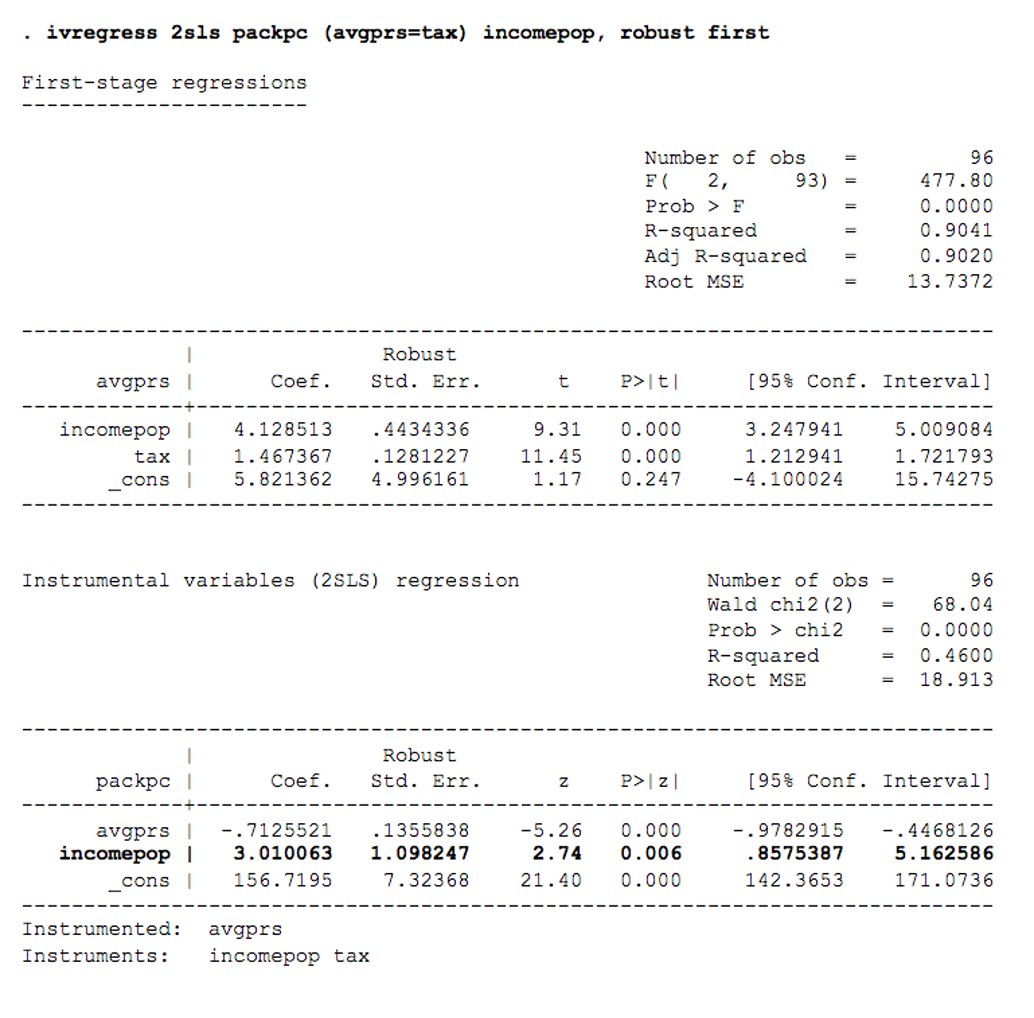
• Even if we have income as a regressor, we still need tax as the excluded instrument
• Stata will give you an error message if there is no excluded instrument

Terminology

• Included instruments: Exogenous regressors (like income) that appear in both stages
• Excluded instruments: Variables (like sales tax) that appear in the first stage but not the second stage
• The “excluded” instrument is what gives IV its identifying power

Panel Data, Fixed Effects, and IV

Combining IV with Panel Data

\[sales_{it} = \alpha_i + \lambda_t + \beta_1 price_{it} + \beta_2 income_{it} + \delta V_i + \omega_{it}\]

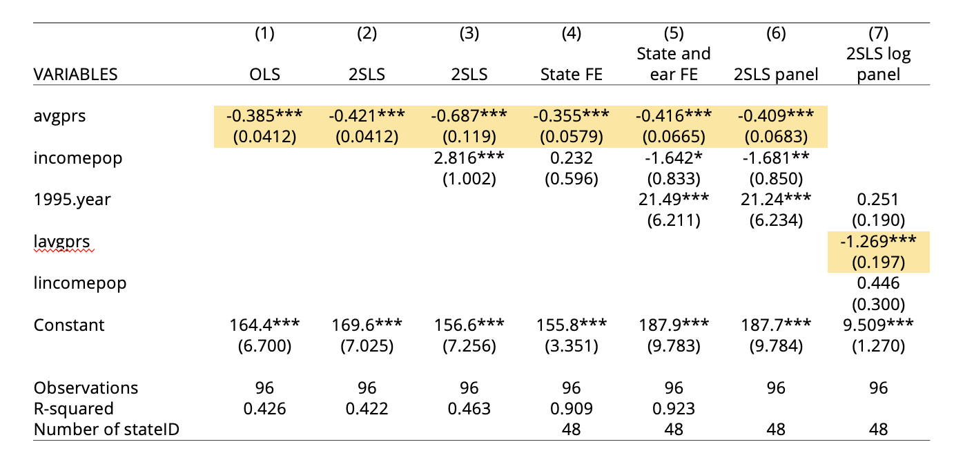
Instrument for price is sales tax (taxs) — the panel-data sales-tax variable; distinct from the per-pack excise tax used earlier.

• Panel data with fixed effects and instrumental variables; data from 1985 & 1995
• State fixed effects (\(\alpha_i\)): Control for time-invariant omitted factors (e.g., a state’s attitude towards smoking)
• Time fixed effects (\(\lambda_t\)): Control for factors affecting all states in one year (e.g., national anti-smoking campaigns)
• Instrument (sales tax): Addresses simultaneous causality between demand factors and price
• Income is assumed exogenous

xtivreg packpc (avgprs = taxs) incomepop y1995, fe vce(cluster state)

Comparing All Specifications

Best Elasticity Estimate

Column 7 adds logs so \(\beta_1\) is an elasticity: when price rises 1%, sales fall 1.3%. The CI of \((-1.53, -1.00)\) lies entirely below \(-1\), so we can reject that demand is inelastic.

What Changes Across Specifications?

Adding state + year FEs and an IV for price (sales tax) moves the coefficient from OLS’s biased estimate toward a credible causal effect.

Applied Example: Returns to Schooling Revisited

A Different Instrument for the Same Problem

We’ve been using wages/schooling throughout. We used distance to college as one instrument. Here’s another famous approach to the same question:

Instrument: Quarter of Birth (Angrist and Krueger, 1991)

• Many states do not let you drop out of school until age 16 (some places 17)
• High school students turn 16 at different times during the year

• Children born earlier in the year can drop out earlier
• So, children born earlier in the year get less total schooling

Check the Three Assumptions

1. Relevant? Yes — quarter of birth is correlated with schooling attainment through compulsory schooling laws
2. Exogenous? Debatable — is quarter of birth correlated with innate ability or other wage determinants? (Bound, Jaeger, and Baker, 1995)
3. Excludable? Debatable — does birth quarter directly affect wages, e.g., through age-at-hire effects?

This instrument has been extensively debated — it illustrates how the assumptions can be challenged even when the research design seems clever.

AK (1991): First Stage

Does quarter of birth actually predict education?

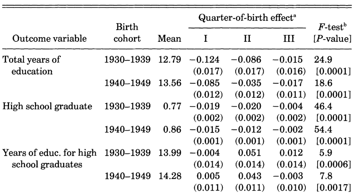
Born in Q1 → significantly less education. F-tests are strong for total years.

AK (1991): The Earnings Pattern

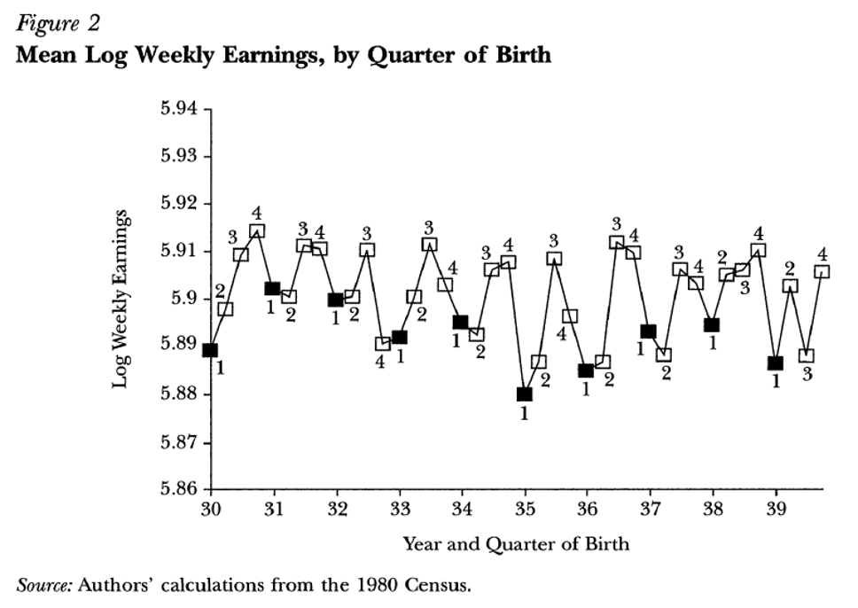
Mean log weekly earnings by quarter of birth (1980 Census). The sawtooth pattern mirrors the education pattern — Q1 births earn less.

AK (1991): OLS vs. TSLS Estimates

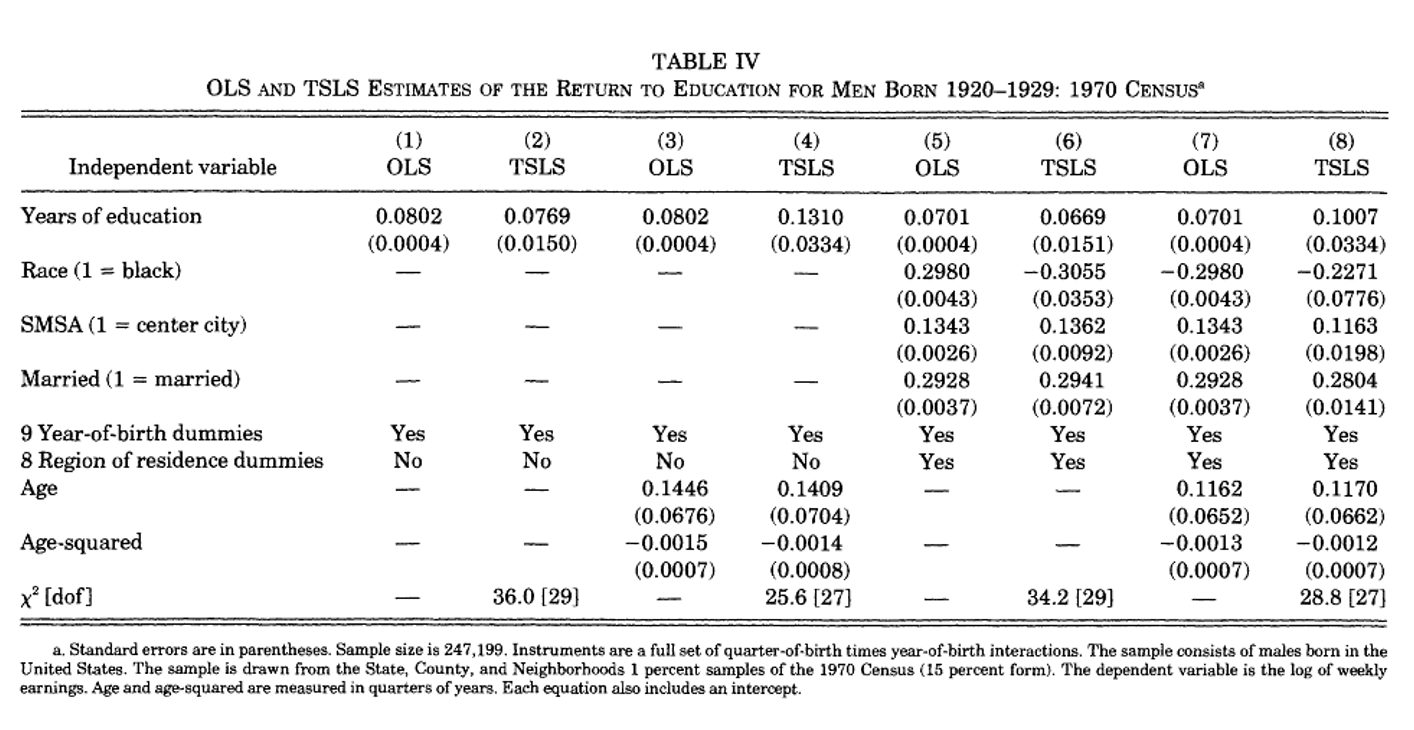
OLS and TSLS estimates of returns to education, men born 1920–1929 (1970 Census, \(n = 247{,}199\)). Instruments: quarter-of-birth × year-of-birth interactions.

Puzzle: IV > OLS?

If ability bias is the main problem, we’d expect OLS to overestimate the return to schooling — so IV should be smaller than OLS. But here IV is larger. Two possible reasons:

• Measurement error in self-reported years of education attenuates OLS toward zero; IV corrects it
• LATE \(\neq\) ATE: compliers here are marginal dropouts, who may have higher returns to each extra year than the average student

Also note: IV standard errors are much larger than OLS — we’re using less variation, so estimates are noisier.

BJB (1995) Problem 1: Inconsistency When the First Stage is Weak

Core insight: When the first stage is weak, even a tiny direct effect of \(Z\) on \(Y\) biases IV more than OLS.

\[\frac{\text{plim}\,\hat\beta_{IV} - \beta}{\text{plim}\,\hat\beta_{OLS} - \beta} \;=\; \frac{\rho_{Z,\varepsilon}/\rho_{X,\varepsilon}}{\rho_{X,Z}}\]

Does QOB have a direct effect on wages? BJB’s quantitative argument:

• Kids born Q1 come from families with 0.024 lower mean log family income (1980 Census)
• Intergenerational income correlation \(\approx 0.4\) \(\Rightarrow\) predicts Q1 wage gap of \(\approx 0.95\%\) from family background alone
• Actual Q1-vs-rest wage gap in AK’s sample: \(\approx 1.1\%\)

BJB’s conclusion

Differences in family income at birth “would seem to account for virtually all of the association between quarter of birth and wages.”

Plus other QOB correlates (school attendance, behavioral problems, reading/writing/math, IQ) — any could open a direct \(Z \to Y\) channel.

BJB (1995) Problem 2: Finite-Sample Bias

Even a legitimate IV is biased toward OLS in finite samples. The magnitude is approximately \(1/F\) — proportional to the first-stage F-stat on the excluded instruments.

For AK’s Q1 \(\times\) year-of-birth specification with within-year age controls (28 excluded instruments): \(F = 1.6\), partial \(R^2 = 0.014\%\). Quantitatively important bias despite \(n = 329{,}509\).

BJB’s smoking gun: replaced AK’s real QOB with randomly-generated “QOB” and re-ran the 2SLS.

	Real QOB	Random noise
Mean 2SLS coef. on educ	0.060	0.061
Mean SE	0.029	0.039
First-stage \(F\)	1.61	\(\approx 1\)
OLS coef (for reference)	0.063	0.063

The lesson

Even with purely random “instruments,” the 2SLS output looks reasonable — point estimate near OLS, plausible SEs. You cannot detect the problem from second-stage coefficients and standard errors alone. Only the first-stage \(F\) reveals it. Always report it.

Why Did AK Use So Many Instruments?

AK’s preferred specification used up to 180 excluded instruments: QOB (3) \(\times\) year of birth (10) \(\times\) state of birth (50) interactions.

The logic (reasonable): Compulsory-attendance laws vary across states (different age cutoffs, different enforcement). So QOB \(\times\) state interactions capture real institutional variation that plain QOB misses — and should also tighten the standard errors.

Why it backfires (BJB’s critique):

• Going from 30 to 178 instruments barely lifts the first-stage \(F\) (4.7 \(\to\) 1.9) and partial \(R^2\) hardly moves — most of the new instruments are weak
• Finite-sample bias scales with \(K/\tau^2 \approx 1/F\) — more weak instruments make the bias worse, not better
• So the extra interactions buy precision without buying identification

Moral

You can’t instrument your way out of a weak first stage by piling on interactions. Quality of instrument variation matters more than quantity of instruments.

IV Recipe Card

IV Estimation: Step by Step

Recipe Card: Instrumental Variables

1. Identify the endogeneity problem

• Why do you think \(\text{Corr}(X, u) \neq 0\)?
• OVB, simultaneous causality, or measurement error?

2. Propose an instrument \(Z\) and argue it is valid

• Powerful: \(\text{Corr}(Z, X) \neq 0\) (testable)
• Exogenous: \(\text{Corr}(Z, u) = 0\) (not testable — must argue)
• Excluded: \(Z\) does not directly cause \(Y\) (not testable — must argue)

3. Estimate via 2SLS

• ivregress 2sls Y (X=Z) controls, robust

4. Report and check

• Report first-stage F-stat (rule of thumb: > 10)
• Discuss threats to exogeneity and exclusion
• Compare IV estimates to OLS — if they differ, explain why

Common Pitfalls

Mistakes to avoid

• Using a weak instrument (F < 10)
• Failing to argue exogeneity
• Forgetting to report the first stage
• Using manual 2SLS standard errors
• Treating IV as a “magic fix” for endogeneity

Good IV practice

• Provide institutional justification for the instrument
• Report the first-stage F-statistic
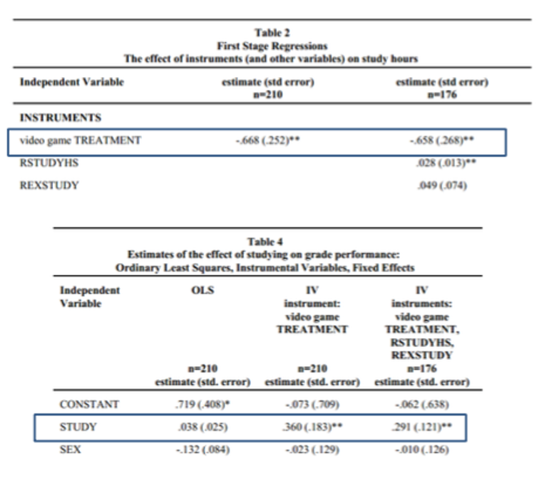
• Use ivregress (not manual two-step)
• Discuss threats to exclusion
• Compare IV to OLS and explain differences

Key Takeaways

1. Endogeneity (\(E(u|X) \neq 0\)) makes OLS biased and inconsistent
2. IV addresses this by finding a variable \(Z\) that:
   • Affects \(X\) (powerful)
   • Is uncorrelated with \(u\) (exogenous)
   • Does not directly affect \(Y\) (excluded)
3. 2SLS isolates the exogenous variation in \(X\) using \(Z\)
4. First-stage F > 10 is a common rule-of-thumb diagnostic for instrument strength
5. Exogeneity cannot be tested — it must be argued
6. IV can be combined with panel data and fixed effects
7. Always use ivregress or xtivreg — never manual two-step

Appendix: Additional Examples

Effect of Studying on Grades

What is the effect on grades of studying an additional hour per day?

• \(Y\) = GPA
• \(X\) = study time (hours per day)

Would you expect the OLS estimator of \(\beta_1\) to be unbiased? Why or why not?

Stinebrickner and Stinebrickner (2008), “The Causal Effect of Studying on Academic Performance,” The B.E. Journal of Economic Analysis & Policy

• \(n = 210\) freshmen at Berea College (Kentucky) in 2001
• \(Y\) = first-semester GPA
• \(X\) = average study hours per day (time use survey)
• Roommates were randomly assigned
• \(Z\) = 1 if roommate brought a video game, = 0 otherwise

Is the Video Game Instrument Valid?

Do you think \(Z_i\) (whether a roommate brought a video game) is a valid instrument?

1. Is the instrument powerful?
   • If your roommate brought a video game, you might study less
   • First stage: video game treatment reduces study hours by 0.67 hours/day (significant)

2. Is the instrument exogenous?
   • Roommates were randomly assigned — so \(Z\) is uncorrelated with unobserved student ability
   • Random assignment makes this a strong argument

3. Is the instrument excludable?
   • Does having a roommate with a video game directly affect your GPA, other than through study time?
   • Plausible: the video game mainly affects grades by reducing study hours

Stinebrickner and Stinebrickner (2008): Results

OLS coefficient on study = 0.038; IV coefficient = 0.36 (much larger). Why? Selection bias — students who study more tend to be weaker students compensating with extra effort (negative selection). IV corrects this by using only the variation in study time driven by the random video-game assignment.