Difference-in-Differences

SW Chapter 10 (Part 2)

ECON3500: Econometrics and Applications

Spring 2026

Quick Review: What We Covered Tuesday

Last class (with Rae), we covered:

Types of data: cross-sectional, time-series, panel, repeated cross-sections
First differencing: $\Delta x_t = x_t - x_{t-1}$ — subtracting periods eliminates time-invariant $\alpha_i$
Fixed effects: give each entity its own intercept ($\alpha_i$)
- Equivalent to demeaning: estimating deviations from each unit’s mean
- Within estimator (FE) vs. between estimator (pooled OLS)

Today: a specific research design built on these tools — difference-in-differences.

The Problem with Simple Comparisons

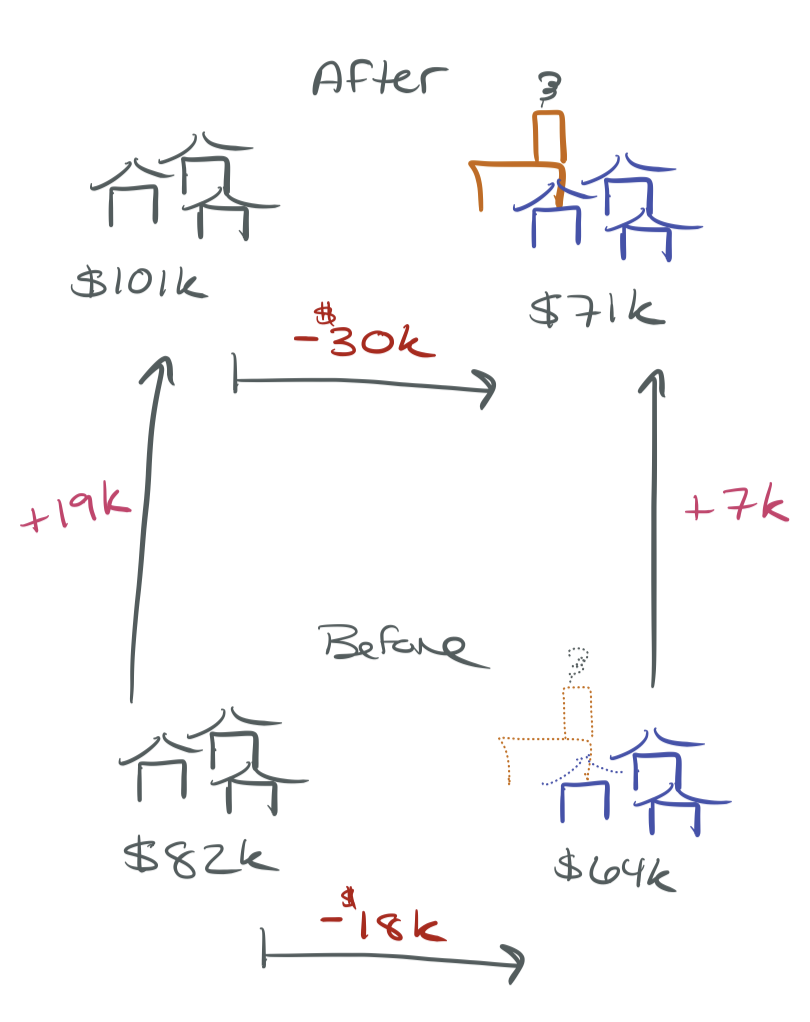
Motivating Example: Garbage Incinerator

Question: What is the effect of a garbage incinerator on nearby housing prices?

After the incinerator was built:

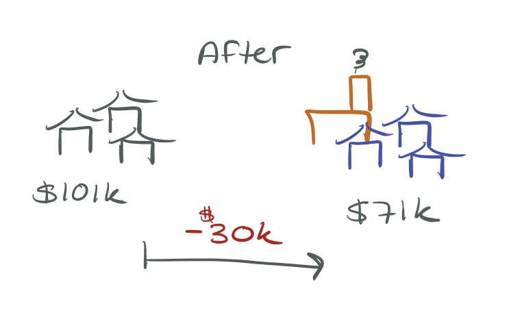
\[\widehat{rprice} = 101{,}308 - 30{,}688 \cdot nearinc\]

Houses near the incinerator sell for ~$30k less. Did the incinerator cause this?

Not So Fast…

Look at the relationship before the incinerator was built:

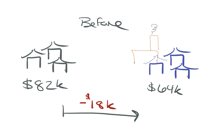
\[\widehat{rprice} = 82{,}517 - 18{,}824 \cdot nearinc\]

The incinerator was built in a place where housing prices were already depressed!

The $30k gap reflects both the incinerator effect and pre-existing differences.

Two Flawed Comparisons

Cross-Sectional Comparison (After Only)

Compare near vs. far houses after the incinerator: $-\$30{,}688$

Problem: Near-incinerator houses were already cheaper. Location characteristics are confounders — they affect both proximity to the incinerator and housing prices.

Before/After Comparison (Treatment Group Only)

Compare near-incinerator houses before vs. after: $+\$18{,}790$

Problem: Housing prices were rising everywhere. We’re mixing the treatment effect with a common time trend.

We need a method that handles both problems simultaneously.

Difference-in-Differences

The Core Logic

Subtract out the pre-existing difference:

\[\begin{aligned} \hat{\delta}_1 &= \underbrace{(-30{,}688)}_{\text{after gap}} - \underbrace{(-18{,}824)}_{\text{before gap}} \\ &= -11{,}864 \end{aligned}\]

The incinerator reduced nearby prices by ~$12k — not $30k.

The 2×2 Table

The difference of differences:

	Before	After	$\Delta$
Control (far)	$82,517	$101,308	+$18,790
Treatment (near)	$63,693	$70,619	+$6,927
Treat $-$ Control	−$18,824	−$30,688	−$11,864

\[\begin{aligned} &\underbrace{(70{,}619 - 63{,}693)}_{\Delta \text{ treat}} - \underbrace{(101{,}308 - 82{,}517)}_{\Delta \text{ control}} \\ &\quad = {\color{red}-11{,}864} \end{aligned}\]

DiD Graphically

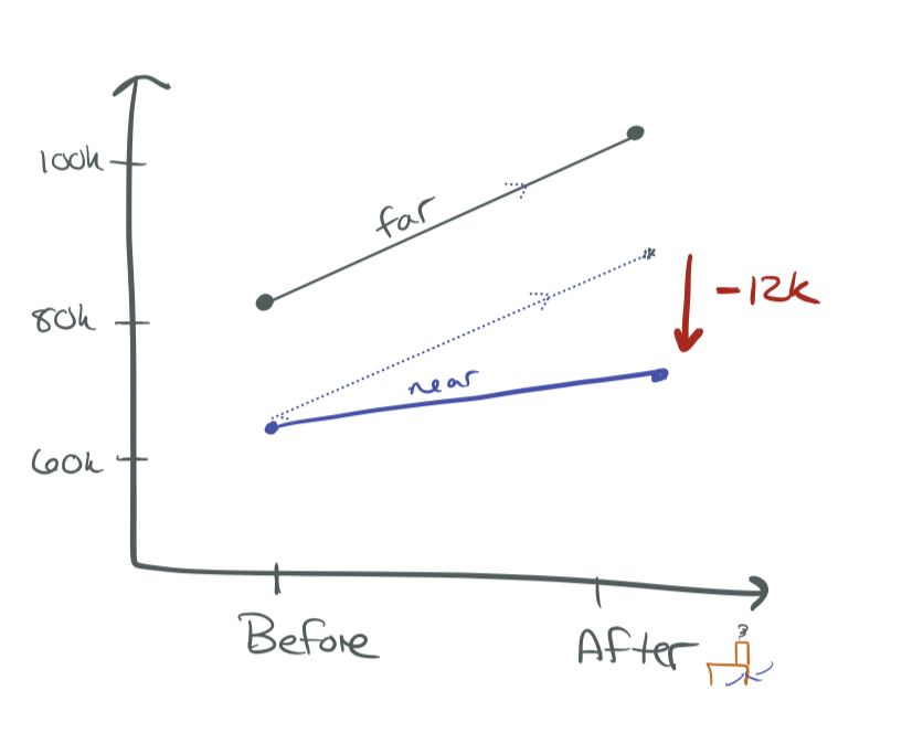
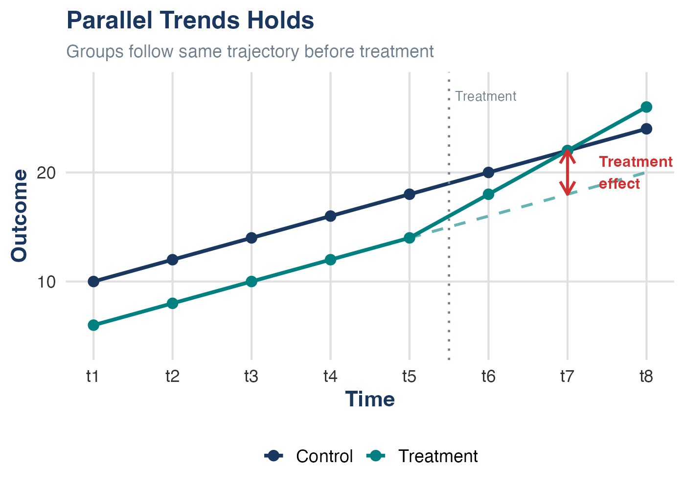
The dashed line shows where near-incinerator prices would have been if they followed the same trend as far-away prices.

The DiD estimate is the vertical gap between:

What actually happened to the treatment group
The counterfactual: what would have happened without treatment

DiD Animated

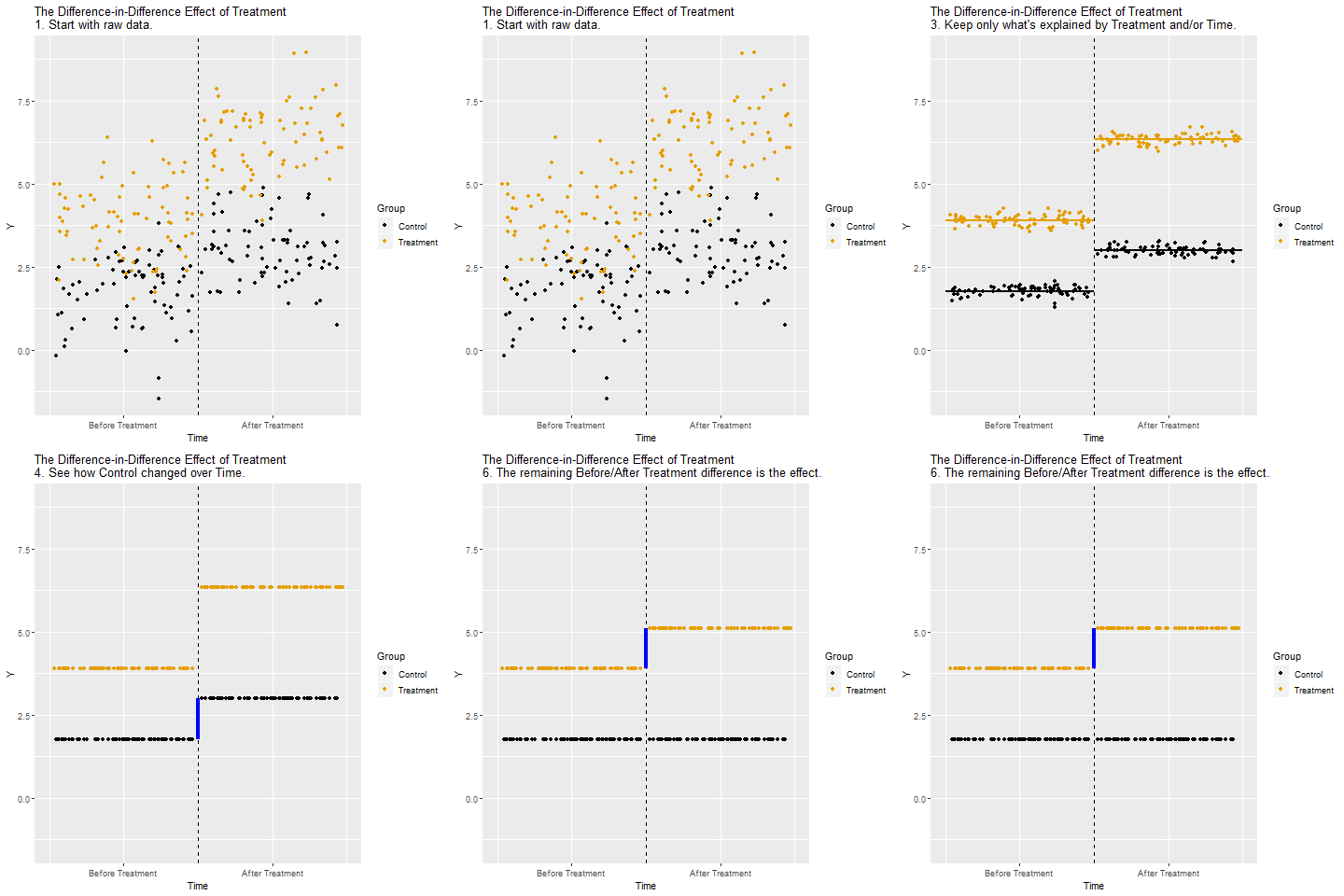
Animation by Nick Huntington-Klein (The Effect)

Watch the steps:

Raw data: two groups over time
Collapse to group means
Measure the control group’s time trend
Subtract that trend from the treatment group
What remains = the DiD estimate

The key: use the control group’s trajectory to build the counterfactual for the treatment group.

The Counterfactual

What DiD Really Estimates

DiD doesn’t compare treatment and control groups directly. It asks:

How much did the treatment group change relative to what would have happened without treatment?

The control group’s trajectory provides the counterfactual — but only if parallel trends holds.

This is why DiD is so useful for policy evaluation:

Treatment and control groups can have very different levels
They just need to be on similar trajectories before the policy hits
The identifying assumption is about trends, not levels

The Regression Framework

DiD as a Regression

We can capture the entire DiD logic in one regression:

\[rprice_i = \beta_0 + \delta_0 \cdot after_i + \beta_1 \cdot nearinc_i + \delta_1 \cdot (after_i \times nearinc_i) + u_i\]

	Before (${\color{white} after = 0}$)	After (${\color{white} after = 1}$)	Change
Control (far)	$\beta_0$	$\beta_0 + \delta_0$	$\delta_0$
Treatment (near)	$\beta_0 + \beta_1$	$\beta_0 + \delta_0 + \beta_1 + \delta_1$	$\delta_0 + \delta_1$
Treat $-$ Control	$\beta_1$	$\beta_1 + \delta_1$	$\delta_1$

$\delta_1$ — the coefficient on the interaction term — is the DiD estimate.

Interpreting Each Piece

\[y_i = \underbrace{\beta_0}_{\text{baseline}} + \underbrace{\delta_0 \cdot after_i}_{\text{time trend}} + \underbrace{\beta_1 \cdot treated_i}_{\text{group difference}} + \underbrace{\delta_1 \cdot (after_i \times treated_i)}_{\text{treatment effect}} + u_i\]

Coefficient	Meaning
$\beta_0$	Average outcome for control group, before
$\delta_0$	How the control group changed over time (common time trend)
$\beta_1$	Pre-existing difference between groups
$\delta_1$	The DiD estimate — causal if parallel trends holds

Adding Control Variables

Why add controls to a DiD regression?

1. Precision: Controls reduce residual variance → tighter standard errors, even if parallel trends holds unconditionally.

2. Credibility: Parallel trends may only hold conditional on covariates. If treatment and control groups differ on observables that predict trends, controlling for those variables makes parallel trends more plausible.

Works fine — just add $\mathbf{X}_{it}$ to the regression:

\[y_{it} = \beta_0 + \delta_0 \cdot after_t + \beta_1 \cdot treated_i + \delta_1 \cdot (after_t \times treated_i) + \gamma' \mathbf{X}_{it} + u_{it}\]

Controls Can Matter for Identification

Unlike in an RCT, parallel trends may only hold after conditioning on observables. Omitting those variables is OVB.

Example: If newer homes were built farther from the incinerator site during this period, controlling for house characteristics isn’t just about precision — it’s about identification.

The Parallel Trends Assumption

The Key Assumption

Parallel Trends Assumption (common trends assumption in SW)

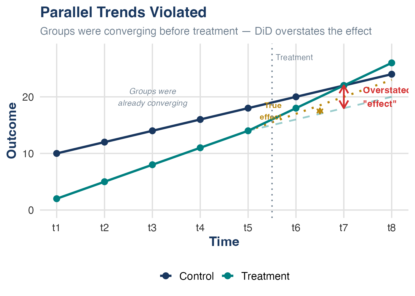
In the absence of treatment, the difference between treatment and control groups would have remained constant over time.

Equivalently: both groups would have followed parallel trajectories.

Key point: Parallel trends is a statement about what would have happened without treatment — it is about the untreated counterfactual, not about what we observe after treatment.

What this allows:

Treatment and control groups can have different levels of the outcome
There can be time-invariant unobserved confounders — DiD differences them out

What this requires:

No time-varying confounders that differentially affect the two groups

Parallel Trends Holds

Groups follow the same trajectory before treatment. The treatment effect is the gap between the actual outcome and the counterfactual (dashed line).

The dashed line = the counterfactual: where the treatment group would have been if it followed the control group’s trend.

Parallel Trends Violated

Groups were converging before treatment. DiD attributes the continued convergence to the treatment — overstating the true effect.

The gold dotted line = the true counterfactual (continuing convergence). The dashed line = what DiD incorrectly assumes. The difference between the two is the bias.

What Would Violate Parallel Trends?

In the incinerator example — what could threaten parallel trends?

A new highway built near the incinerator site at the same time
A neighborhood revitalization program targeting the area
Differential migration (people leaving because the incinerator was announced)

More generally, any factor that:

Changes over time (not absorbed by entity or time FE)
Affects treatment and control groups differently
Coincides with the timing of treatment

Assessing Parallel Trends

We can never prove parallel trends — it’s about what would have happened without treatment.

But we can look for supporting evidence:

1. Pre-treatment trend test: Plot the outcome for both groups over time. Do they move in parallel before treatment?

2. Placebo/falsification tests:

Run DiD using a fake treatment date (before the real one). A significant “effect” suggests something else is driving the result.
Run DiD on an outcome that should not be affected by treatment.

3. Event study plot: Estimate treatment effects for each period relative to treatment. Pre-treatment coefficients should be near zero and flat.

The Event Study Plot

An event study estimates separate effects for each period relative to treatment:

\[y_{it} = \alpha_i + \lambda_t + \sum_{k \neq -1} \delta_k \cdot D_{it}^k + u_{it}\]

where $D_{it}^k = 1$ if unit $i$ is $k$ periods from treatment at time $t$.

Think of it as DiD estimated separately for each time period — revealing when effects emerge and whether they grow, fade, or were already present before treatment.

What to look for:

Pre-treatment coefficients ($k < 0$): Should be close to zero → supports parallel trends
Post-treatment coefficients ($k \geq 0$): Show the dynamic treatment effect over time
The reference period ($k = -1$) is normalized to zero

Why Event Studies Matter

Event study plots have become nearly mandatory in applied DiD papers. They are the most credible way to support — though not necessarily prove — the parallel trends assumption.

Real-World Example

Card & Krueger (1994): Does the Minimum Wage Kill Jobs?

Question: Does raising the minimum wage reduce employment?

Setting:

New Jersey raised its minimum wage from $4.25 to $5.05 in April 1992
Pennsylvania did not change its minimum wage
Surveyed fast-food restaurants in both states, before and after

	Before	After	Δ
NJ (treatment)	20.44 FTE	21.03 FTE	+0.59
PA (control)	23.33 FTE	21.17 FTE	−2.16
NJ − PA			+2.76

Result: Employment increased in NJ relative to PA — the opposite of the standard prediction. One of the most influential papers in labor economics.

Why Is Card & Krueger Compelling?

What makes this a good DiD design?

Sharp treatment: NJ raised the minimum wage on a specific date; PA didn’t
Geographic neighbors: NJ and PA share economic conditions → plausible parallel trends
Same industry: Fast food in both states faces similar demand shocks
No obvious differential shocks: No major PA-specific event in 1992 that would have changed fast-food employment

What might you be concerned about?

Were NJ restaurants anticipating the wage increase? (announcement effects violate sharp timing)
Did PA have its own employment shocks unrelated to the minimum wage?
Are the two states similar enough for parallel trends?
Measurement error: Employment data came from phone surveys of managers

DiD in Stata

Estimating DiD

Option 1: Interaction regression

* Generate interaction term
gen after_treat = after * treated

* Estimate DiD
reg y after treated after_treat, robust

Option 2: Factor variable notation (preferred)

* Stata creates the interaction automatically
reg y i.after##i.treated, robust

The coefficient on 1.after#1.treated is the DiD estimate $\hat{\delta}_1$.

DiD with Panel Data in Stata

With true panel data (same entities over time), combine DiD with fixed effects:

* Set panel structure
xtset entity_id year

* Entity + time FE with DiD
xtreg y treated_post i.year, fe vce(cluster entity_id)

Or equivalently, using reghdfe:

reghdfe y treated_post, absorb(entity_id year) vce(cluster entity_id)

Don’t Forget to Cluster!

With panel data, always cluster standard errors at the entity level — we’ll cover exactly why on Tuesday.

Wrapping Up

DiD and Internal Validity

Ch 9 Threat	How DiD Helps	What DiD Cannot Fix
OVB	Eliminates time-invariant confounders by differencing	Time-varying confounders that differentially affect groups
Wrong functional form	Flexible — can add covariates, nonlinearities	Misspecified treatment timing or group definitions
Measurement error	Not addressed	Attenuation bias still applies
Sample selection	Not addressed	Differential attrition (people move because of treatment)
Simultaneous causality	Treatment timing helps	If treatment is responsive to anticipated outcomes

DiD Checklist

Before you trust a DiD estimate, ask:

Is there a clear treatment group and control group?
Is there a clear before and after period?
Is parallel trends plausible? What evidence supports it?
Are there pre-trend tests or an event study plot?
Could any time-varying confounder have changed differentially at the same time?
Are standard errors clustered appropriately? (we’ll discuss why on Tuesday)

Key Takeaways

DiD combines a cross-sectional comparison with a time comparison — the causal interpretation requires parallel trends
The interaction term captures the DiD estimate ($\hat{\delta}_1$)
Parallel trends is untestable — it’s about a counterfactual — but pre-trends and event studies provide supporting evidence
DiD addresses time-invariant OVB by differencing it out — but time-varying confounders that differentially affect groups still threaten validity
Always cluster standard errors at the entity level with panel data — more on this Tuesday

	Before (\({\color{white} after = 0}\))	After (\({\color{white} after = 1}\))	Change
Control (far)	\(\beta_0\)	\(\beta_0 + \delta_0\)	\(\delta_0\)
Treatment (near)	\(\beta_0 + \beta_1\)	\(\beta_0 + \delta_0 + \beta_1 + \delta_1\)	\(\delta_0 + \delta_1\)
Treat \(-\) Control	\(\beta_1\)	\(\beta_1 + \delta_1\)	\(\delta_1\)