Lab 3: Regression

Due by 1:15 pm on Thursday, February 12, 2026

Lab Content

Download these and save in your lab folder (perhaps you named it something like econ3500/labs?)

👁️ If your do-file opens in a browser tab, you may want to instead right click and select “Save Link As” 👁️

Before you start

Set your working directory in Stata to the folder where you saved the data and template.
Start a log file right away: log using lab3.log, replace
Make sure you can open the dataset with use graduation.dta, clear.

By the end of this tutorial you should be able to complete the following tasks in Stata:

Estimate and interpret a simple (two-variable) linear regression in levels, using continuous and binary variables, and use heteroskedasticity-robust standard errors.
Identify $\hat{\beta_0}$, $\hat{\beta_1}$, standard errors, $SST$, $SSE$, $SSR$, and $R^2$ in Stata output and interpret them
Calculate predicted values and residuals
Create scatter plots
Estimate a multivariate linear regression

command	description
Estimation commands
`regress var1 var2`	Estimate a regression, with `var1` as the dependent variable and `var2` as the independent variable(s)
`regress var1 var2, robust`	Estimate a regression with heteroskedasticity-robust standard errors
`correlate var1 var2 ... varn`	Calculate correlation coefficients of all listed variables, from `var1` to `varn`.
`graph twoway scatter var1 var2`	make a scatter plot with `var1` on the y-axis and `var2` on the x-axis.
Post-estimation commands¹
`predict newvar, xb`	Use estimated regression coefficients to predict $\widehat{y}$. It will generate `newvar`²
`predict newvar, residuals`	Use estimated regression coefficients to predict residuals, generating `newvar`³
Working with data, missing values
`count if var1 == 1`	count observations if the expression `var1 == 1` is true
`count if !missing(var1)`	count observations if `var1` is not missing
`drop if missing(var1)`	drop all observations where `var1` is missing
`tab var1, missing`	Include missing values in tabulation

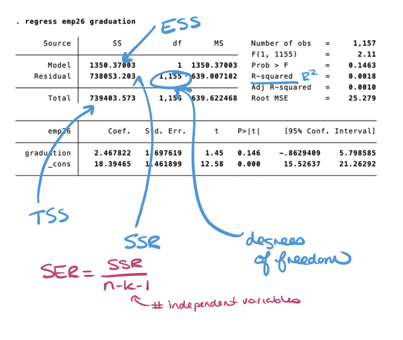
Quick reminders

The coefficient estimates do not change when you add , robust.
The standard errors do change when you add , robust.
Run predict immediately after your regression. If you run another command in between, Stata will overwrite the stored model.

Your written answers to exercise questions (1) - (13). This can be typed or written out then scanned (or photographed), in any reasonable format.
The do-file you’ve created that runs this analysis
A log file that contains the results from this exercise.

Today, we’re going to look around at the graduation data set that we discussed in class, graduation.dta.

Download the do-file template and data files. Personalize the file paths so that you can run it and open your graduation.dta file. You can also work with a blank data file if you’re more comfortable - just make sure you remember to include commands to start and close your log file.
Take a look at graduation.dta. How many observations are there? What is the distribution of treatment arms?⁴
There are six continuous food security variables⁵. You can look for them with lookfor fs. Pick one variable and write out a population model to determine the relationship between assignment to the graduation program and food security. For the rest of this lab, I refer to the variable you chose as foodsecurity. If that’s going to irritate you, you can rename your variable like this: rename fsec5 foodsecurity, using the variable name that you’ve chosen in place of fsec5.
Tabulate your food security value and check for missing observations. Drop any observations for which you have missing values of foodsecurity (see above for how to do this). How many observations are remaining?

Hint After you drop missing values, run count to confirm your new sample size. Keep that number consistent for the rest of the lab.

Make a scatter plot of the relationship between your chosen food security variable and graduation (Include this in your submitted problem set). Is this easy to interpret? Calculate and report the associated correlation coefficient.
Conduct a t-test of whether the mean of foodsecurity is different between those who did and did not receive the graduation program⁶
Estimate the relationship between your chosen food security variable, foodsecurity and assignment to the graduation program, graduation using simple linear regression, with standard (homoskedasticity-assumed) standard errors. How do your t-statistics compare to what you found in the previous t-test? What was the impact of assignment to the graduation program on food security, based on your regression?
Re-estimate your regression, and this time adjust your standard errors to be heteroskedasticity-robust. Fill in the chart below with your estimates.

Variable	Estimate	Variable	Estimate
$\hat{\beta_0}$		$\hat{\beta_1}$
$R^2$		$TSS$
$ESS$		$SSR$
d.f.		$SER$

After that regression estimate, generate a new variable, predict_fs equal to the predicted value of your food security variable. Generate a second variable, resid_fs equal to the residual.
What is the mean of each variable? How does the mean of predict_fs compare to mean of foodsecurity in your sample?⁷
Examine the predicted value of your food security variable, predict_fs, for the youngest person in your sample.⁸ What is its residual?
When we estimate a linear regression with no coefficients, sometimes we’ll say we are “regressing on a constant.” Regress foodsecurity only on a constant. What is $\hat{\beta_0}$, and how does it compare to overall mean?
For this final step, I’d like you to play around with the data. Pick one continuous dependent variable and one continuous or binary independent variable.⁹ You can look at the correlation between two variables, or you can look at the impact of one of the program dimensions (group coaching, group livelihood, etc) on a continuous outcome of interest.

a. Write a population model you want to estimate.

b. Estimate it using OLS, adjusting your standard errors to be heteroskedasticity-robust. Write an equation that reflects your estimated model in the form $\hat{y}=\hat{\beta_0} + \hat{\beta_1}x$, replacing $y$ and $x$ with your chosen variables and replacing $\hat{\beta_0}$ and $\hat{\beta_1}$ with your estimates.

c. In 1-2 sentences, what do your results tell you, collectively?

Submission checklist

Post-estimation commands must be run immediately after a regression, while the regression results are still held in your local variables. ↩︎
Here, newvar equals $\widehat{newvar_i} = \widehat{y_i} = \widehat{\beta_0} + \widehat{\beta_1}x_i$ ↩︎
Here, newvar equals $\widehat{newvar_i} = \widehat{u_i} = y_i - \left(\widehat{\beta_0} + \widehat{\beta_1}x_i\right)$ ↩︎
There are a few variables here, including treatment_arm ↩︎
Not fsec7, which is categorical, or fsec which is always equal to 1 ↩︎
Hint: ttest var1, by(var2) will run a t-test of whether the mean of var1 is equal for two groups determined by var2. ↩︎
If they differ, you should make sure you have dropped all missing values of foodsecurity! Try sum predict_fs foodsecurity to see if the sample sizes are the same ↩︎
Now is a good time to try out lookfor age ↩︎
Categorical variables that take on a just few observations, like the identity of your head of household, won’t work here. You’ll need to tabulate the variables to see what you’re working with ↩︎

Last updated on February 17, 2026