Lab 1: Introduction to Stata
Download print-friendly version (pdf)
Materials
Objectives1
By the end of this tutorial you should be able to complete the following tasks in Stata:
- Identify key areas of the Stata interface
- Open a data file
- Understand what a working directory is
- Summarize and tabulate data
- Make a variable
- Create and save a log file
- Open, view, and save a data file
- Ask Stata for help
If you need more help, check out Stata Resources.
For the hardcore R users in this class who prefer to use R throughout, you may complete this lab in R. But, it could also be fun to learn a little Stata!
General command structure
do {something} ... with {variable(s) x}...if {something is true..}, options
Note: In this lab, you may type commands directly into the Command window. Later in the course, we will use do-files, which allow you to save and rerun your code. For now, your log file will serve as a record of your work.
Key commands
| command | description |
|---|---|
log using logfile1.log |
open and log using logfile1.log |
log close |
close log |
use dataset.dta, clear |
open dataset dataset.dta , clear out old one |
describe var1 var2 ... |
charcteristics of var1, var2, etc. |
browse var1 var2 ... |
open data browser, display var1, var2 .. |
lookfor text1 |
search for text1 in variable names/descriptions |
tabulate var1 |
make a frequency table of var1. |
tabulate var1 var2 |
make a cross-tabulation of var1 and var2. |
summarize var1 |
descriptive statistics for var1. |
summarize var1 , detail |
detailed descriptive statistics for var1. |
gen var1 = binexp |
generates a variable var1 equal to 1 if binary expression true, 0 otherwise |
replace var1 = 0 if binexp |
replaces var1 to be 0 if binary expression true, nothing otherwise |
help command |
open help files for command. |
Logic statements
These are some common logical statements
| operation | command |
|---|---|
| and | & |
| or | | (vertical bar, on same key as “/") |
| equal to | == |
| not equal to | != |
| greater than | > |
| less than | > |
| greater than or equal to | >= |
| less than or equal to | <= |
-
tab bac10 if gdl==1 & sl70plus == 0- Tabulates the variable
bac10but only ifgdlequals one andsl70plusequals 0
- Tabulates the variable
-
tab bac10 if year >=2000- Tabulates the variable
bac10for the years 2000, 2001, 2002, etc.
- Tabulates the variable
-
tab bac10 if year !=2000:- Tabulates the variable
bac10for every year but 2000
- Tabulates the variable
-
tab bac10 if year < 2008 & year > 2005- Tabulates the variable
bac102006 and 2007
- Tabulates the variable
-
tab bac10 if year < 2008 | year > 2005- Tabulates the variable
bac10is less than 2008 OR greater than 2005 (all years!)
- Tabulates the variable
Also: you can use parentheses to group terms appropriately. For example, if you want to tabulate states where the speed limit is 55 or 65 AND the blood alcohol limit is 0.10, then this is wrong:
tab state if sl55 == 1 | sl65 == 1 & bac10 == 1
But this is correct!
tab state if (sl55 == 1 | sl65 == 1) & bac10 == 1
Thanks, parentheses!
Guided instructions
Hey, Stata. It’s nice to meet you
Start by opening Stata. You should have a window that looks something like this (on a PC):
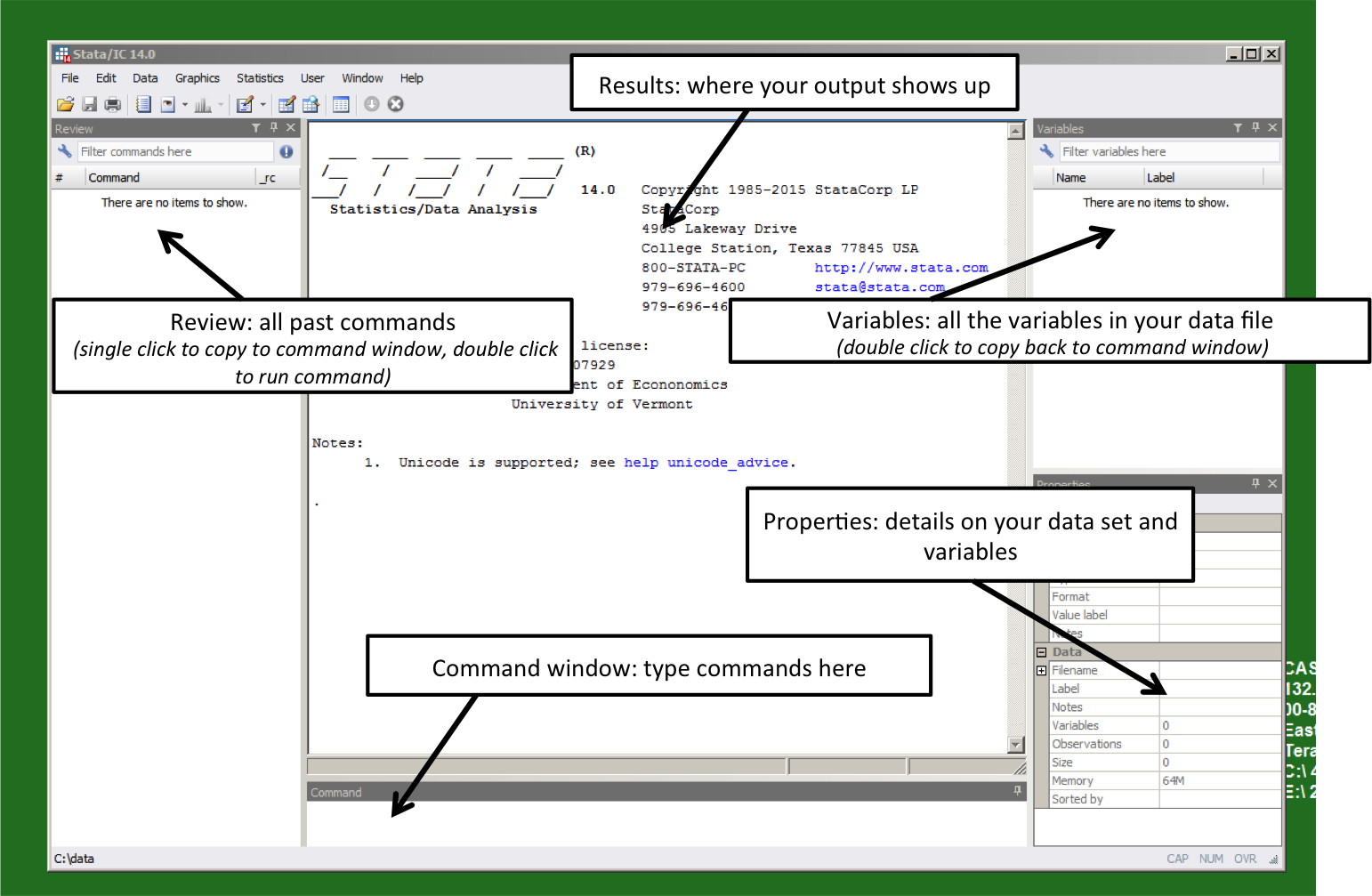
You should now have the Stata window open. There is a set of pull down menus as well as 4 smaller windows: Review, Variables, Results, and Command.
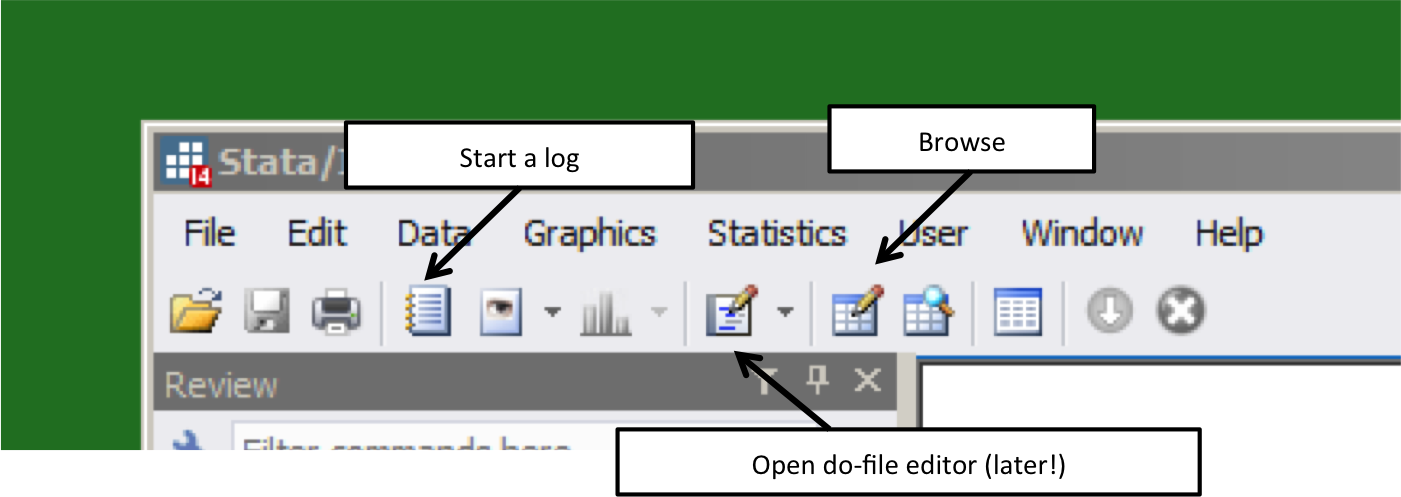
Also especially helpful are the following buttons:
Log files
If you want to record anything that you do in a Stata session so that you can look at results or commands later, you need to open a log-file. A log-file is simply a record of all the commands you enter into Stata and the output from those commands. The key is to make sure you have a log file open at the beginning of a Stata session, and to close it once you have finished, and before you close Stata.
There are three ways you can open a log file:
-
Go to the FILE dropdown menu, choose Log, choose Begin. You should see a “Begin Logging Stata Output” dialog box. Browse to a directory where you can store your log file and type in the following file name in the File Name space:
lab1.log -
Click on the log icon at the top of the Stata workspace (right of the print button). When you click on the log button, the “Begin Logging Stata Output” dialog box pops up. Name your log file as above.
-
You can open a log file by typing the following in the Stata command window:
log using lab1.log, replaceThe
, replaceis optional. If you add it as an option, your new file will overwrite your old one. Or, you can add, appendto add it to the bottom of your old log file.
Tip: Use extension .log, NOT the default .smcl. This will make it easier for you to edit, cut and paste your log in any text editor.
Now that you have a log file open, we can start our STATA session.
Working directories (important!)
Stata looks for data files in its working directory. To see your current working directory, type:
pwd
If your data file is not located there, Stata will not find it. You can change your working directory using:
cd "/path/to/your/folder"
Once you run this command, Stata will make this working directory its starting point, but only for the rest of the session. The next time you open Stata, you may need to repeat the process.
I recommend creating a folder for this class (e.g., econ3500/labs/) and saving both your data and log files there.
Opening data files
Stata data files end with the extension .dta, and they can only be
read by Stata. You can import text files and excel files into Stata, and
you can export .dta files into text files or Excel files, but we’ll
cover this later.
There are three ways to open a data file:
-
Outside Stata, double click on the data file you want to open
-
Use the FILE/OPEN drop down menu in Stata and open the data set that you copied into your folder. Note that in the command window, the
usecommand appears. We’ll use that one later. -
Type
use filename.dta, clearinto the command window within Stata. The option, cleartells Stata to remove any data currently in memory. Stata can only hold one dataset at a time.2
Download
driving_2004.dta and open it. I recommend moving it to your brand new class folder first. It is a
file of driving laws, vehicle accidents, and fatalities in the United
States in 2004.
You should now see the list of variables appear in the Variables window, with the variable name, variable label, and some other information.
Looking at data
Let’s take a more detailed look at the variables in the dataset.
In the command window type: describe
At the top of the output you will see some overall features of the file,
including the number of variables. Below that you will see a list of
every variable, including the variable name, the “storage type” (byte,
float, int, etc.) and the variable label. If you see –more– at the
bottom of your screen, press the space bar to continue scrolling.3
To learn more about the variables and the organization of the data, use
the browse command. Type: browse (or click on the “browse” button).
Another approach is to add a variable list to the browse command. Type the following:
browse year sl70plus bac10 bac08 gdl
Again, note that you can also double click on the variable names so you don’t have to type them all!
This command directs you to a spreadsheet inside Stata where the data appears. This looks a lot like an Excel spreadsheet!
Note the following:
-
Each observation appears on a separate row of the spreadsheet, which represents data from a certain year and a certain state. For example the first row is for state 1 (Alabama) in 1980. If you move along the row, you can see other characteristics about Alabama in 1980.
-
Each variable appears in a separate column, and the name of the variable is at the column heading.
How many observations are there? What type of data set is this?
Examining variables
Let’s look at the variables that are included in the data set. There is an efficient way to find the names of variables you are interested in. Suppose you are interested in a variable related to alcohol laws. Type in:
lookfor alcohol
This will give you a list of all the variables that have “alcohol” in
either their variable name or variable label. In this case, two
variables appear - bac10 and bac08.
You can also experiment with all possible combinations of the col, row,
and cell options, and add the nofreq option to suppress the number of
observations. Use help for details:
help tab
When you are analyzing variables, you will want to think carefully about whether you should be looking at row percentages, column percentages, or cell percentages.
Creating new variables
You can create new variables using the generate command. For example:
gen highfatal = fatal_rate > 1.5
This creates a variable equal to 1 when the condition is true, and 0 otherwise.
You could create the same variable in a slightly different way:
gen highfatal = 1         if fatal_rate > 1.5
  replace highfatal = 0   if fatal_rate < 1.5
Videos
Lab Exercise 1
First, work through the above steps. Then, work through the 7 questions below.
What do I submit?
- Your written up answers to exercise questions (1) - (7). This can be typed or written out then scanned (or photographed), in any reasonable format
- A log file that contains the results from the steps prior to the exercise and the exercise itself.
If you struggled or explored, this might get excessively long! Three choices (1) submit it anyways, (2) open it in a text editor manually delete the nonsense, (3) close your log file and start a new one, and this time run through your code with less backtracking. Option (1) is completely fine.
Questions
-
How many states have graduated drivers license laws (GDLs)? How many states have speed limits of 70 mph or higher (including no speed limit)?
-
What percentage of states with GDLs and with low speed limits (below 70 mph) have blood-alcohol limits of 0.10 (the more lenient level)? Note that some states have blood-alcohol limit for a fraction of a year. If so, consider having a limit of 0.10 in place for part of the year as having a limit
-
What is the mean fatality rate per 100 million miles across all states? What is the standard deviation?
-
What was the fatality rate (deaths per 100 million miles) in Vermont? (Vermont is state 46)
-
Generate a variable $Y$ equal to one if a state has a fatality rate per 100 million miles that is above the mean, and zero otherwise. What is $E(Y)$?
-
Write a joint probability distribution table for the following two random variables: $X$, a random variable equal to one if a state has a speed limit of 70 or greater and zero otherwise (see
sl70plus), and $Y$, the random variable developed in the previous part. -
Look up the command
correlatein the help files: What is the correlation coefficient between nighttime fatalities per 100,000 population and weekend accidents per 100,000 population? Why might this correlation be so strong?
-
This lab draws heavily on Anne Fitzpatrick’s (UMass-Boston) excellent materials. ↩︎
-
Yes, this is a pain. ↩︎
-
If you are tired of dealing with the “more” issue, you can enable
set more offinto the command window to enable continuous scrolling for your session. If you’re just done with it, tryset more off, permto enable continuous scrolling for this and all future sessions. ↩︎